🌀 AUC — Analytical Ultracentrifugation
Analytical Ultracentrifugation (AUC) measures how macromolecules redistribute in a centrifugal field. It is powerful because the experiment is performed in free solution: no column matrix, immobilization surface, or label is required for standard absorbance and interference detection. The key outputs are sedimentation coefficients, concentration distributions, buoyant molar masses, and model-dependent estimates of molar mass and shape.
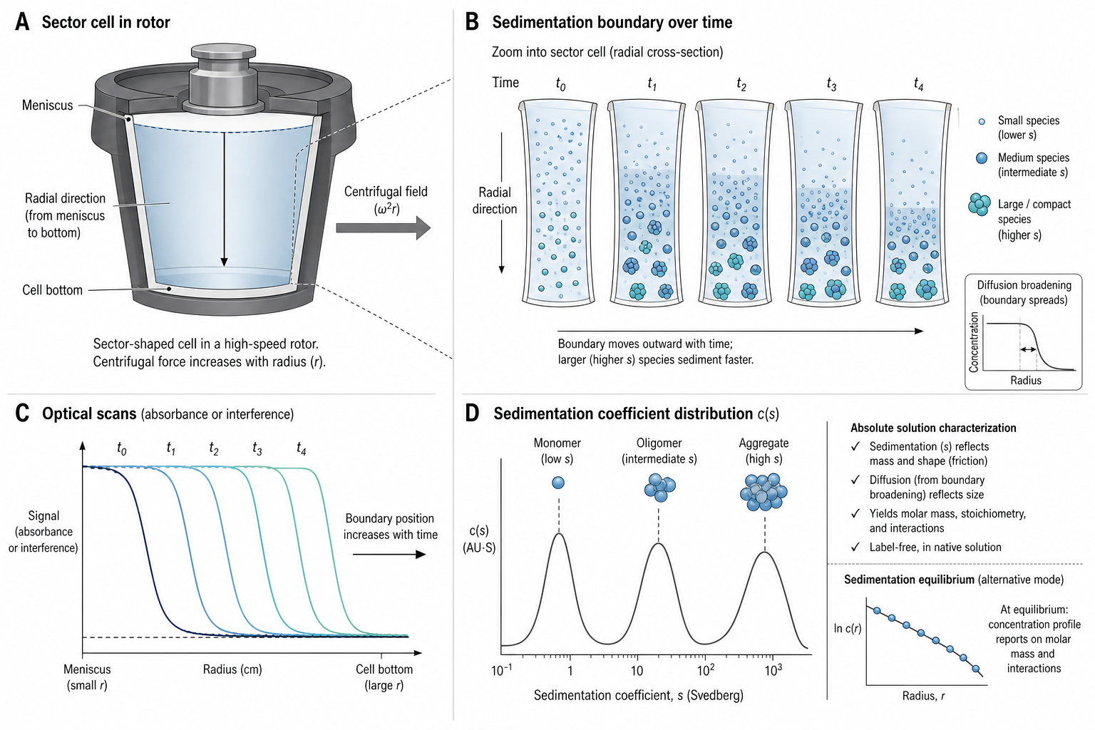
AUC comes in two flavors: Sedimentation Velocity (SV-AUC) spins at high speed (40,000–60,000 rpm). Molecules sediment toward the cell bottom at rates determined by their mass, shape, and density. Record the moving boundary over time with absorbance or interference optics. Fit the data with the Lamm equation to estimate a sedimentation coefficient distribution, most commonly c(s). Molar mass can be inferred only when diffusion or frictional information is supplied by the model; it is not a direct readout of SV data. A typical SV-AUC experiment takes 4–12 hours.
Sedimentation Equilibrium (SE-AUC) spins at lower speed (5,000–25,000 rpm, with the low end set by MW for very large complexes) until sedimentation and diffusion reach a thermodynamic equilibrium. The resulting concentration gradient depends on buoyant molar mass, concentration, and association model, but not on hydrodynamic shape. SE-AUC can determine shape-independent molar mass for well-behaved species when partial specific volume and solvent density are known, and can measure weak self-association KD values when the loading concentrations span the association transition. SE-AUC takes 12–72 hours to reach equilibrium. Separately, fluorescence-detected AUC (FDS-AUC) is an optical detection upgrade usable in SV experiments; tracer experiments such as NUTS/BOLTS can extend binding measurements to very tight affinities, but require labeled material and careful control experiments.
When do you need AUC? When DLS can't resolve your species (Rh ratio < 3:1, a rule of thumb that depends on intensity contributions), when SEC-MALS shows column interactions, when you need sedimentation coefficients or hydrodynamic heterogeneity in solution, or when an orthogonal higher-order-structure method strengthens a comparability package. AUC is slower and more expertise-intensive than DLS or SEC-MALS, so it is best reserved for questions where solution-state separation by sedimentation actually changes the answer.
Key Physics Concepts
The Svedberg Equation
In a centrifugal field, a molecule sediments under the effective buoyant force and is opposed by solvent friction. At steady boundary motion, the sedimentation coefficient s links radial velocity to field strength:
s = u / (ω²r) = (dr/dt) / (ω²r) = M(1 − v̄ρ) / (NA f)Combining this with the Einstein relation D = RT/(NA f) gives the Svedberg equation. It converts s and D into molar mass only when both transport coefficients refer to the same species:
M = s × R × T / (D × (1 − v̄ρ))- s = sedimentation coefficient (1 S = 10⁻¹³ s)
- u = dr/dt = radial migration velocity of the boundary
- v̄ = partial specific volume (mL/g; ~0.73 for proteins)
- ρ = solvent density (g/mL; ~1.00 for water)
- D = diffusion coefficient (m²/s)
- f = frictional coefficient
- M from SV is model-dependent unless D is independently constrained
| Molecule | MW (kDa) | s₂₀,w (S) |
|---|---|---|
| RNase A | 13.7 | 1.85 |
| Lysozyme | 14.3 | 1.9 |
| BSA (monomer) | 66.5 | 4.3 |
| BSA (dimer) | 133 | 6.6 |
| IgG | 150 | 6.5–7.0 |
| IgM (pentamer) | 950 | 19 |
| Ribosome (70S) | 2500 | 70 |
Frictional Ratio f/f₀ — Shape Information
The frictional coefficient f tells you about shape. Compare it to f₀, the friction of a smooth sphere of the same mass:
R_min = (3Mv̄ / (4πNA))^(1/3)Key insight: f/f₀ combines hydration and asymmetry. A perfectly spherical protein with the typical ~0.3 g water/g protein hydration layer has f/f₀ ≈ 1.10–1.15; observed values of 1.2–1.3 reflect combined hydration plus minor non-sphericity. Values above 1.3 indicate genuine elongation.
| f/f₀ | Interpretation |
|---|---|
| 1.0 | Perfect anhydrous sphere (theoretical) |
| 1.2–1.3 | Globular, hydrated protein (typical) |
| 1.4–1.6 | Moderately elongated or flexible (IgG) |
| 1.7–2.0 | Highly elongated |
| > 2.0 | Rod-like, intrinsically disordered, or strongly asymmetric (fibrinogen ~2.3–2.5) |
c(s) Distribution — Resolving Species
The c(s) distribution is the primary output of many sedimentation velocity analyses. It is a distribution over sedimentation coefficient, not a mass spectrum: two species with the same s can have different molar masses if their shapes or buoyancies differ. The Lamm equation describes the transport:
∂c/∂t = (1/r) ∂/∂r [r(D ∂c/∂r − sω²rc)]Programs such as SEDFIT and UltraScan fit Lamm-equation models to many scans simultaneously, estimating distributions across a grid of sedimentation coefficients with regularization or model-selection constraints.
Resolution advantage: SV-AUC can resolve many mixtures that DLS averages together, but the practical resolution depends on signal-to-noise, scan spacing, concentration, boundary separation, and the fitted model. Compare:
- DLS: rule of thumb — can't resolve species with Rh ratio < ~3:1 (~27× volume; depends on intensity contributions)
- SEC-MALS: column plate count limits (~1.5× MW)
- c(s): closely spaced species may require high-quality data and appropriate regularization; a monomer/dimer pair with a large Δs is much easier to resolve than near-isomeric or conformationally similar species
Molecule Parameters
Preset
Reading the chart
Each curve is an f/f₀ isocontour — for the same MW (y-axis), a more elongated molecule (higher f/f₀) sediments slower (lower s, moves left). s alone does not determine MW; you need shape information (f/f₀) or diffusion (D).
MW vs s₂₀,w — f/f₀ isocontours (log–log)
White dot = current selection. Curves from left to right: f/f₀ = 1.0 (sphere) → 2.0 (elongated). v̄ = 0.730 mL/g.
SV-AUC — How It Works (Practical)
⚗️ Experimental Setup
- Sample preparation. 0.2–1.0 mg/mL protein, 400–450 µL in 12 mm path-length cells (or 100 µL in 3 mm cells). Higher concentration → better S/N but risks non-ideal behavior and self-association.
- Reference sector. Fill with matching buffer. Both sample and reference sectors must be at the same meniscus height.
- Rotor speed. 40,000–60,000 rpm for proteins <100 kDa. Slower (25,000–40,000 rpm) for larger complexes (>500 kDa) to prevent pelleting before enough scans are collected.
- Temperature equilibration. Pre-equilibrate at run temperature (typically 20°C) for 1–2 hours with the rotor at rest. Temperature gradients during acceleration create convection artifacts.
- Detection. Absorbance (280 nm for proteins, 260 nm for nucleic acids) or interference (Rayleigh). Interference is label-free and linear over a wider concentration range.
- Run duration. 200–400 scans over 4–12 hours. Resolution improves when the boundary is sampled well across time and radius; simply collecting more scans is not a substitute for appropriate speed and scan timing. Ensure the boundary reaches at least ⅔ of the cell length.
📊 Data Analysis
- Load data. Import scans into SEDFIT, UltraScan, or equivalent Lamm-equation software. Define the meniscus and bottom positions carefully — wrong boundaries bias fitted s-values and residuals.
- Set parameters. Buffer density ρ, buffer viscosity η, partial specific volume v̄ (use 0.73 mL/g for proteins unless measured; calculate from sequence with SEDNTERP).
- Fit a transport model. c(s), 2DSA, or related models fit many scans simultaneously. Regularization/model selection controls how much structure is allowed in the distribution.
- Check residuals. Should be random. Systematic residuals indicate: wrong meniscus, non-ideality, time-invariant noise, or inappropriate model.
- Read c(s). Identify peaks, integrate for s₂₀,w and relative abundance. Treat molar masses and f/f₀ values as model-dependent estimates unless supported by independent diffusion, known stoichiometry, or orthogonal measurements.
- Report. s₂₀,w, c(s) distribution plot, relative percentages of species, model assumptions, residuals, and any molar-mass or shape estimates with their assumptions.
SE-AUC — How It Works (Practical)
⚗️ Experimental Setup
- Loading. 100–120 µL per channel at 3 concentrations (e.g., 0.2, 0.5, 1.0 mg/mL) and 2–3 rotor speeds. Multiple concentrations and speeds help test whether a single model explains the data and can improve parameter confidence when the model is identifiable.
- Speed selection. Choose so that the signal at the cell bottom is ~5–10× the signal at the meniscus. Rule of thumb: σ(r_bottom² − r_meniscus²)/2 ≈ 2–5, where σ = M(1−v̄ρ)ω²/(RT) (matches the c(r) exponent below).
- Equilibration. 12–48 hours (sometimes longer for large complexes or at low speeds). Check by overlaying consecutive scans — equilibrium is reached when scans don't change.
- Short-column method. Use 50–70 µL to shorten equilibration time. It can be useful for simple single-species molar-mass checks, but gives less radial information for heterogeneity or association models.
- Detection. Absorbance often preferred for SE because concentration is directly measured (needed for thermodynamic analysis of self-association KD).
📈 Data Analysis
- Global fit. Fit multiple speeds and concentrations simultaneously in SEDPHAT, UltraScan, or equivalent software. Single-ideal-species model: c(r) = c₀ exp[σ(r²−r₀²)/2] + baseline.
- Self-association models. Monomer-dimer, monomer-dimer-tetramer, and isodesmic models require global parameters such as monomer molar mass and association constants plus local parameters such as loading concentrations, baselines, and extinction/signal factors. The concentration and speed dependence of the radial profiles constrains KD.
- Buoyant molar mass. Primary output is Mb = M(1−v̄ρ). To get true M, you need v̄ — measured or calculated from sequence (SEDNTERP).
- Non-ideality. At high concentrations (>1 mg/mL for large proteins), the second virial coefficient BM becomes significant. Global fitting with non-ideality corrections is possible in SEDPHAT.
- Precision. For a single well-behaved species, SE-AUC can give precise buoyant molar mass. For self-associating systems, KD precision depends on the concentration range, speed range, signal calibration, reversibility, and whether the model is identifiable.
Partial Specific Volume (v̄) — The Critical Parameter
v̄ determines the buoyancy factor (1 − v̄ρ). If v̄ is wrong, molar-mass estimates that depend on buoyancy are wrong.
| Macromolecule | v̄ (mL/g) |
|---|---|
| Proteins (average) | 0.73 ± 0.02 |
| Glycoproteins (20–30% glycan) | 0.70–0.72 |
| Nucleic acids (DNA) | 0.55 |
| Nucleic acids (RNA) | 0.53 |
| Detergent micelles (DDM) | 0.82 |
| PEG | 0.836 |
| Lipids | 0.90–1.00 |
How to determine v̄
- From amino acid sequence. Calculate using SEDNTERP (Cohn & Edsall amino acid volumes). Accuracy ±0.01 mL/g for unmodified proteins.
- From density measurements. Measure solution density at multiple solute concentrations and derive v̄ from the density increment after consistent unit conversion. This can be accurate, but requires more material and careful matched-buffer measurements.
- From solvent contrast variation. Compare sedimentation in solvents with different densities to estimate the effective buoyancy of complexes whose composition is not known from sequence alone, such as protein-detergent or glycoprotein systems. D₂O experiments must account for H/D-exchange and density/viscosity changes; H₂¹⁸O can avoid exchange artifacts but is more specialized.
Common Pitfalls
Wrong meniscus position
In SV-AUC, the meniscus is the air-liquid boundary. A wrong meniscus can bias fitted s-values, broaden distributions, and create systematic residuals. Meniscus fitting can help, but verify the fitted boundary manually.
Temperature not equilibrated
Temperature gradients create convection — especially in the first 30 minutes after acceleration. Pre-equilibrate the rotor at run temperature for 1–2 hours. If you see "wavy" residuals in early scans, discard them.
Concentration too high → non-ideality
Above ~1 mg/mL for large proteins (>100 kDa), hydrodynamic non-ideality (governed by the coefficient k_s) shifts a single species' apparent s downward. Run multiple concentrations and extrapolate to c→0. This is distinct from the multi-component Johnston-Ogston effect (see pitfall #7).
Assuming v̄ = 0.73 for everything
Fine for unmodified globular proteins but wrong for glycoproteins (0.70–0.72), DNA (0.55), RNA (0.53), detergent complexes (variable), or PEGylated proteins. Calculate from sequence (SEDNTERP) or measure.
Over-interpreting c(s) peaks
Small peaks at unexpected s-values can be artifacts, model regularization effects, time-invariant noise, systematic errors in early/late scans, or meniscus artifacts. A real species should be reproducible, physically plausible, and supported by residuals.
Not running enough scans
SV resolution improves when the boundary is sampled well over time and radius. Too few scans, poor scan timing, or a boundary that pellets too early can make distinct species merge into one broad distribution.
Neglecting the Johnston-Ogston effect
In concentrated interacting or multicomponent systems, transport coupling and hydrodynamic non-ideality can distort apparent boundary areas and s-values. Do not treat peak area percentages as absolute composition without checking concentration dependence and model assumptions.
Absorbance non-linearity above OD 1.2
Absorbance becomes non-linear above ~1.2 OD. Interference detection is linear over a much wider range. For heterogeneous samples with high-MW aggregates, interference is preferred.
Strengths & Limitations
| ✅ Strengths | ❌ Limitations |
|---|---|
| Solution-state sedimentation analysis — no column, surface, or label for standard optics | Expensive instrument (~$300–800K new Beckman Optima; ~$150–250K used XL-I) |
| Can resolve sedimentation heterogeneity that DLS averages together | Specialized expertise required (not a walk-up instrument) |
| Hydrodynamic shape information through model-dependent f/f₀ estimates | Long run times: SV 4–12 h, SE 12–72 h |
| Weak self-association analysis in native solution when concentrations span the transition | High sample consumption: 400–450 µL per 12 mm cell at ~0.5 mg/mL (less for short-path cells) |
| No column artifacts (unlike SEC-MALS) | Limited throughput: 3–7 samples per run |
| Broadly applicable to soluble macromolecules, assemblies, viruses, and dispersed particles when signal and stability are adequate | Requires accurate v̄ — error propagates to MW |
| Useful orthogonal method for comparability and higher-order-structure packages | Data analysis requires training and careful model selection |
| Sensitive to small sedimenting species when signal-to-noise and optics are adequate | Cannot work with very turbid or precipitating samples |
When NOT to Use AUC
❌ For routine QC screening
DLS takes 2 minutes; AUC takes hours. For daily QC of protein preps, use DLS or SEC-MALS. Reserve AUC for definitive characterization.
❌ When you need high-throughput
AUC runs 3–7 samples at a time. If you have 100 formulation conditions to screen, use DLS plate reader (384-well in 30 min) or SEC-MALS with an autosampler.
❌ For very small molecules (< ~5 kDa)
Small peptides and small molecules sediment very slowly and give tiny signals. The s-values overlap with buffer component sedimentation.
❌ For membrane proteins without knowing the complex v̄
The effective v̄ of a protein-detergent complex is not predictable from sequence alone. Without measuring v̄ (e.g., by D₂O contrast), MW will be wrong. Alternative: SEC-MALS with protein conjugate analysis.
❌ When your sample precipitates during the run
AUC runs are hours long. If the protein is marginally stable, it may aggregate during the experiment. Check DLS and DSF stability first. Run at 4°C if needed.
❌ For equilibrium K_D of tight binders (< ~µM) without FDS
Standard absorbance/interference SE-AUC measures K_D only when the accessible concentration range spans the binding transition. Fluorescence-detected tracer SV-AUC can reach much tighter affinities, but it is a specialized labeled experiment rather than a default SE replacement.
AUC vs Related Techniques
🌀 AUC (SV)
- Separates by sedimentation in centrifugal field
- c(s) reports sedimentation-coefficient distributions
- Molar mass and f/f₀ are model-dependent unless independently constrained
- 4–12 hours per run, ~400 µL
- No column or surface artifacts
- Best for: oligomeric characterization and hydrodynamic shape constraints
⚖️ SEC-MALS
- Separates by size exclusion column
- Absolute MW from light scattering (independent of shape)
- 30–60 min per run, 20–100 µg
- Column interactions can shift elution
- No shape information (unless combined with viscometry)
- Best for: routine MW verification, oligomeric state
💫 DLS
- Measures diffusion → Rh (no separation)
- Very fast (2–5 min), 10–50 µL
- Intensity-weighted → biased toward large species
- Poor resolution for mixtures (rule of thumb: needs ~3:1 diameter ratio)
- No MW (estimated from Rh empirically)
- Best for: quick aggregation screening, QC
🧲 Native MS
- Exact mass → exact stoichiometry
- Identifies which subunits are in each complex
- MS-compatible buffer required (ammonium acetate)
- Not quantitative for populations
- No shape information
- Best for: subunit composition, complex stoichiometry
Publication Checklist
SV-AUC
- ☐Instrument stated (Beckman Optima, rotor type)
- ☐Rotor speed (rpm) and temperature stated
- ☐Detection system (absorbance wavelength or interference)
- ☐Sample concentration and buffer composition stated
- ☐Cell path length stated (3 mm or 12 mm)
- ☐Number of scans and scan interval
- ☐v̄ value stated with source (sequence-calculated or measured)
- ☐Software stated (for example SEDFIT or UltraScan, including analysis settings)
- ☐c(s) distribution plot shown
- ☐s₂₀,w values for each species ± SD
- ☐Molar-mass/f/f₀ estimates reported only with model assumptions
- ☐Residuals shown (bitmap or RMSD value)
- ☐Relative percentages of species reported
SE-AUC
- ☐Rotor speeds (multiple speeds recommended)
- ☐Loading concentrations (multiple recommended)
- ☐Equilibrium verification method stated (scan overlay)
- ☐Model stated (single-species, monomer-dimer, etc.)
- ☐v̄ value stated with source
- ☐Software stated (for example SEDPHAT or UltraScan)
- ☐Buoyant molar mass or molar mass ± confidence interval with v̄ source
- ☐K_D ± confidence interval for self-association
- ☐Residuals shown
- ☐Radial concentration profiles shown
General
- ☐Buffer density and viscosity stated or referenced
- ☐Temperature stated and equilibration time
- ☐s₂₀,w correction applied (not raw s_obs)
- ☐If non-ideal conditions: virial coefficient or c→0 extrapolation noted
- ☐Comparison to orthogonal technique (SEC-MALS, DLS) when possible
Key References
- Cole, J. L., Lary, J. W., Moody, T. P. & Laue, T. M. Analytical Ultracentrifugation: Sedimentation Velocity and Sedimentation Equilibrium. Methods Cell Biology 84, 143–179 (2008). Practical foundation for SV and SE experiment design, transport equations, and interpretation.
- Brown, P. H., Balbo, A. & Schuck, P. A Practical Introduction to Sedimentation Velocity Analytical Ultracentrifugation. Current Protocols in Immunology 81, 18.15.1–18.15.39 (2008). Source for the c(s), Lamm-equation, and reporting guidance used here.
- Schuck, P. Size-distribution analysis of macromolecules by sedimentation velocity ultracentrifugation and Lamm equation modeling. Biophysical Journal 78, 1606–1619 (2000). Seminal c(s) and regularized Lamm-equation modeling paper.
- Brown, P. H. & Schuck, P. Macromolecular size-and-shape distributions by sedimentation velocity analytical ultracentrifugation. Biophysical Journal 90, 4651–4661 (2006). Defines why c(s)-derived mass and shape estimates are model-dependent.
- Demeler, B. & Gorbet, G. E. Analytical Ultracentrifugation Data Analysis with UltraScan-III. In Analytical Ultracentrifugation: Instrumentation, Software, and Applications, 119–143 (Springer, 2016). Basis for including UltraScan, 2DSA, genetic algorithms, and HPC workflows alongside SEDFIT/SEDPHAT.
- Kingsbury, J. S. & Laue, T. M. Fluorescence-detected sedimentation in dilute and highly concentrated solutions. Methods Enzymology 492, 283–304 (2011). Background for FDS-AUC and tracer binding experiments.
- Beckman Coulter. Optima AUC product specifications. Manufacturer source for current instrument optics and rotor descriptions.
Instruments for AUC
Instruments
- Beckman Coulter Optima AUC — current flagship; UV-visible absorbance and Rayleigh interference optics; 8-hole (An-50 Ti) or 4-hole rotors
- Beckman Coulter ProteomeLab XL-I — previous generation; absorbance + interference; still widely used
- Nanolytics MWL-AUC detector — multi-wavelength add-on for Beckman Optima/XL-I; resolves spectrally distinct components in a complex
- Aviv FDS module — fluorescence-detected AUC add-on; enables tracer SV-AUC experiments with very low fluorescent concentrations
Software
- SEDFIT (Peter Schuck, NIH) — c(s) analysis, Lamm equation modeling; free download
- SEDPHAT (Peter Schuck, NIH) — global analysis, SE-AUC fitting, multi-method integration; free
- SEDNTERP — buffer density/viscosity calculator, v̄ from sequence; free
- UltraScan-III — alternative to SEDFIT with 2DSA and genetic algorithm optimization, global fitting, and HPC workflows
- Optima AUC analysis software — vendor-provided acquisition and analysis tools; useful for instrument workflows, not a replacement for expert model selection
- GUSSI — graphical utility for AUC data visualization and c(s) plotting
Have SPR or BLI data?
Upload your raw files and get an automated kinetic analysis in minutes. We support Biacore, Octet, and other major formats.
Upload & Analyze