💫 DLS & SEC-MALS — Size, Aggregation, and Molecular Weight

Figure 1 schematic explaining DLS and SEC-MALS: light scattering geometry, intensity autocorrelation to hydrodynamic radius, SEC separation with MALS and RI detectors, and size and molar-mass outputs

Before you measure binding, you need to know what you're measuring is actually what you think it is. Is your protein a monomer or an aggregate? Is it monodisperse or a heterogeneous mess? DLS and SEC-MALS answer these questions — they're the quality control gatekeepers that belong upstream of every binding experiment.

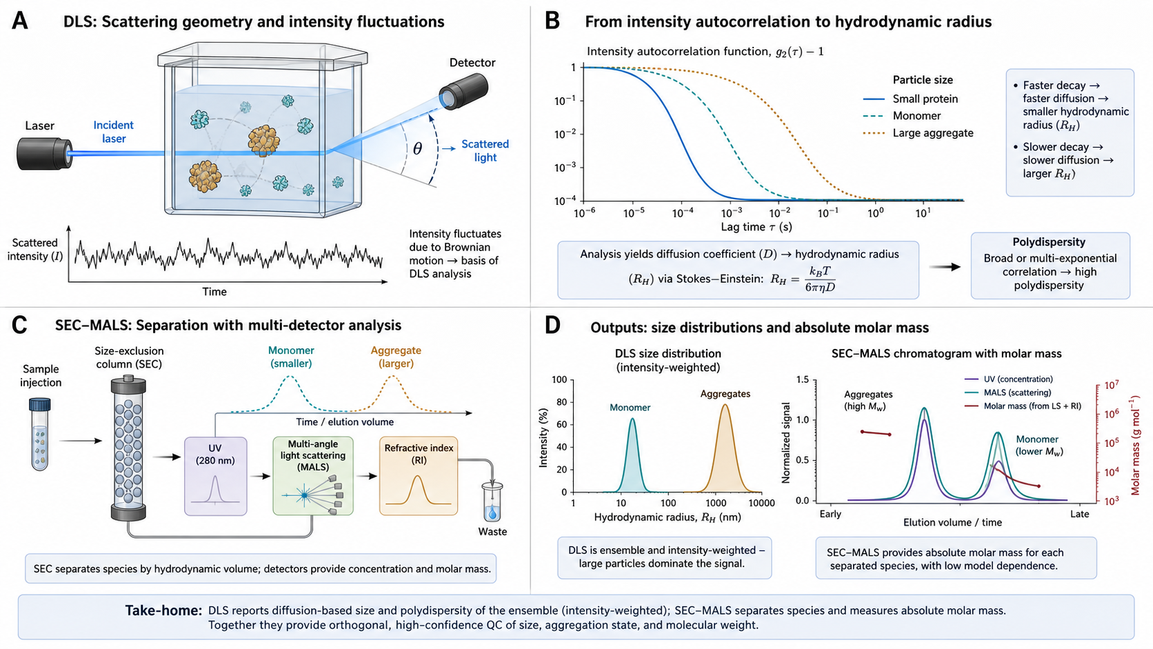
DLS (Dynamic Light Scattering) measures hydrodynamic size by watching how fast particles jiggle in solution. Shine a laser, measure the flickering of scattered light, compute the autocorrelation function → diffusion coefficient → hydrodynamic radius via the Stokes-Einstein equation. Takes 2–5 minutes per sample, needs ~10 µL. If your DLS shows polydispersity or aggregation peaks, stop — fix your protein before wasting reagents on SPR/ITC/MST.

SEC-MALS (Size Exclusion Chromatography with Multi-Angle Light Scattering) goes further: it separates species by size (SEC column) and then measures the absolute molecular weight of each peak from the angular dependence of scattered light intensity. Unlike plain SEC-UV, which estimates MW from elution volume relative to standards, SEC-MALS gives you the actual MW independent of shape or conformation. This is how you prove your "monomer" peak really is a monomer and not a compact dimer.

Neither DLS nor SEC-MALS measures binding affinity. They answer "what is it?" and "how big is it?" — not "how tight does it bind?" Use these upstream, then move to SPR, MST, ITC, or FP for K_D.

Key Physics Concepts

🔬

Brownian Motion & The Stokes-Einstein Equation

Particles in solution undergo Brownian motion — random jiggling driven by thermal energy from solvent molecules. Smaller particles diffuse faster; larger particles diffuse slower.

D = k_BT / (6π η R_h)

D = translational diffusion coefficient (m²/s)
k_B = Boltzmann constant (1.381 × 10⁻²³ J/K)
T = absolute temperature (K)
η = solvent viscosity (Pa·s; water at 25°C: 8.9 × 10⁻⁴ Pa·s)
R_h = hydrodynamic radius (m)

Key insight: DLS doesn't measure size directly — it measures D, which is converted to an equivalent sphere radius R_h. For elongated or flexible molecules, R_h overestimates the minimum dimension.

Molecule	MW (kDa)	R_h (nm)
Insulin (monomer)†	5.8	1.3
Lysozyme	14.3	1.9
BSA	66.5	3.5
IgG (antibody)	150	5.3
IgM (pentamer)	950	12.5
Ribosome (70S)	2500	~13
Liposome (100 nm)	—	50

† Insulin R_h shown for the theoretical monomer. In solution at typical DLS concentrations, insulin exists as a dimer or (with Zn²⁺) as a hexamer — the species you actually observe depends heavily on Zn²⁺ and concentration.

📊

DLS — The Autocorrelation Function

DLS measures the autocorrelation of scattered light intensity over time:

g⁽²⁾(τ) = 1 + β × |g⁽¹⁾(τ)|²

Where β is the coherence factor (0.5–0.95) and the decay rate Γ = D × q² with scattering vector q = (4πn/λ₀) × sin(θ/2).

Cumulant analysis expands ln|g⁽¹⁾(τ)| as a polynomial — the first cumulant gives the z-average D, the second cumulant gives the PDI.

PDI	Quality
< 0.1	Monodisperse — ideal
0.1–0.25	Narrow — acceptable
0.25–0.5	Broad — investigate
> 0.5	Very broad — unreliable

⚖️

SEC-MALS — Absolute Molecular Weight

SEC-MALS couples three in-line detectors: UV (280 nm), refractive index (RI), and multi-angle light scattering (MALS). The Rayleigh-Debye-Gans equation:

K × c / R(θ) = 1/(M_w × P(θ)) + 2A₂c

Where K = 4π²n₀²(dn/dc)² / (N_A × λ₀⁴). For most globular proteins (R_g < 10–15 nm), P(θ) ≈ 1, so:

M_w = R(θ) / (K × c)

This gives the absolute MW at each point across the chromatogram — no shape assumption, no standards needed. Correct for glycoproteins, PEGylated proteins, membrane protein-detergent complexes.

Sample Parameters

Hydrodynamic Radius (R_h)nm5.0 nm

PDIpolydispersity index0.05

Temperature°C25°C

R_h5.0 nm

D4.91 × 10⁻¹¹ m²/s

Γ3.41e+4 s⁻¹

η (water)0.890 mPa·s

PDI0.05

QualityMonodisperse

MW (est.)175 kDa

Physics reminder

The decay shifts right as R_h increases — larger particles diffuse slower (smaller D, smaller Γ). PDI broadens the transition: high PDI means a mixture of sizes, each decaying at a different rate.

g⁽²⁾(τ) − 1 vs. log₁₀(τ / s)

x-axis: log₁₀ delay time (s). β = 0.8 (coherence factor). θ = 173°, λ₀ = 633 nm, n = 1.33.

DLS Measurement — Practical Guide

⚗️ Sample Preparation

Filter or centrifuge. Remove dust and large aggregates with a 0.02–0.1 µm filter (PVDF or PES; 0.1 µm is a minimum — 0.02 µm gives cleaner baselines) or centrifuge at 16,000g × 10 min. Dust particles scatter enormously and ruin the measurement.
Concentration: 0.1–10 mg/mL for proteins. Higher → better scattering signal, but interparticle interactions affect D above ~5 mg/mL.
Buffer: Avoid high concentrations of fluorescent compounds or absorbing species. The laser (633 nm typically) shouldn't be absorbed. Colorless buffers are ideal.
Temperature equilibration: Allow 2–5 min for equilibration before measurement. Temperature gradients cause convection → artificially small R_h.
Cuvette/capillary: Use disposable cuvettes (ZEN0040 for low volume) or flow-through capillary. Clean reusable cuvettes with filtered water/ethanol.
Repeat measurements: Run at least 3 measurements per sample. Check that R_h and PDI are consistent — drift suggests aggregation, sedimentation, or temperature instability.

📊 Measurement & Analysis

Set correct solvent parameters. Viscosity and refractive index must match your buffer. Glycerol, sucrose, or PEG significantly increase viscosity — if not corrected, R_h will be overestimated.
Attenuator and count rate. Too high → detector saturation. Too low → poor statistics.
Cumulant analysis. Use for quick z-average and PDI. Reliable when PDI < ~0.3 (ISO 22412:2017 guidance); above this threshold use regularization methods (CONTIN, NNLS, or REPES).
Number vs. intensity distribution. Report the intensity distribution (primary data). Use number distribution only qualitatively — it requires assumptions about optical properties.
Multiple scattering check. At concentrations >10 mg/mL, multiple scattering can occur → apparent R_h decreases. Dilute and re-measure. Backscatter geometry (173°) is less sensitive.
Correlogram quality check. The autocorrelation function should start at ~0.8–0.95 and decay smoothly to 0. Noisy or non-decaying correlograms indicate poor sample quality.

SEC-MALS — Practical Guide

⚙️ System Setup

Column choice: Superdex 75 (3–70 kDa), Superdex 200 (10–600 kDa), Superose 6 (5–5000 kDa). Match column range to your protein MW.
Flow rate: 0.5 mL/min typical. Slower → better resolution but longer run.
Detector order: Column → UV → MALS → RI. RI is placed last because its larger cell volume causes more band broadening; this effect is minimized at the end of the flow path.
Calibration: Normalize MALS detectors using an isotropic scatterer (BSA monomer, ~3.5 nm << λ/20). Corrects for detector geometry and inter-detector normalization.
Inject: 20–100 µg protein in 50–100 µL. For MW precision: use 50 µg minimum.
Buffer equilibration: Run buffer baseline until RI is stable (30–60 min). RI baseline drift → systematic MW error.

📈 Data Analysis

Peak selection. Define integration limits for each peak. Avoid including void volume (V₀) aggregates unless you want to measure them.
Band broadening correction. Inter-detector band broadening smears the alignment between UV, MALS, and RI signals. Software corrects using the BSA calibration peak.
MW calculation. At each time slice, MW = R(θ) / (K × c). The MW across the peak should be flat (constant) for a monodisperse species.
dn/dc. Use 0.185 mL/g for unmodified proteins. For glycoproteins, PEGylated proteins, or membrane protein-detergent complexes, determine dn/dc experimentally or use conjugate analysis.
MW precision. Typically ±1–5% for well-behaved proteins. Degrades for very small proteins (<10 kDa) or very large complexes.
R_g from MALS. For particles with R_g > ~10–15 nm, angular dependence gives R_g from a Zimm or Debye plot.

What DLS & SEC-MALS Tell You (and What They Don't)

Parameter	DLS	SEC-MALS
Hydrodynamic radius (R_h)	✅ Primary output	❌ (couple with viscometer)
Molecular weight (MW)	⚠️ Estimated from R_h (assumes globular)	✅ Absolute (from light scattering)
Polydispersity (PDI)	✅ From cumulant analysis	✅ From MW across peak
Oligomeric state	⚠️ Inferred from R_h	✅ Direct (MW = N × monomer MW)
Radius of gyration (R_g)	❌	✅ For particles >10 nm
Shape information	⚠️ R_h only (equivalent sphere)	⚠️ R_g/R_h ratio (if combined with DLS)
Aggregation detection	✅ Excellent (r⁶ sensitivity)	✅ Good (SEC separates + MALS measures)

What they DON'T measure: Binding affinity (K_D) — use SPR, MST, ITC, FP. Binding kinetics (k_on/k_off) — use SPR, BLI. Secondary structure — use CD, FTIR. Thermal stability (T_m) — use DSF, CD, DSC. Stoichiometry of complexes — use native MS for subunit composition.

DLS for Protein Quality Control

This is the most important practical application — and why DLS belongs in a biophysics curriculum.

🔍 The DLS QC Decision Tree

Measure DLS on your protein preparation (2 min)
Check z-average R_h: Does it match the expected value? (See empirical correlation at right.)
- R_h >> expected: aggregation or oligomerization
- R_h << expected: degradation/fragmentation
Check PDI:
- PDI < 0.1: Proceed with binding experiments
- PDI 0.1–0.25: Acceptable, note in publication
- PDI > 0.25: Investigate — run SEC to separate species
Check for multiple peaks:
- Single peak: Good
- Peak at >100 nm: Aggregates present — filter or re-purify
- Peak at <1 nm: Buffer artifact

🌡️ DLS as a Thermal Shift Orthogonal

Some DLS instruments (Malvern Zetasizer, NanoTemper Prometheus Panta) support thermal ramps → measure R_h vs. temperature → detect onset of aggregation (T_agg) as a sharp R_h increase.

This complements nano-DSF T_m: a protein can unfold at 60°C but not aggregate until 75°C, or vice versa. T_m and T_agg can differ significantly — both matter for formulation and stability.

Minimum R_h from MW (globular proteins, Erickson 2009):

R_min (nm) = 0.066 × M(Da)^1/3

R_min is the radius of an anhydrous sphere of equivalent mass; measured R_s = (f/f_min) × R_min, with f/f_min ≈ 1.2–1.3 for typical globular proteins (accounts for hydration and shape). Use as a sanity check, not a primary MW method. Ref: Erickson (2009) Biol. Proced. Online 11:32, Eq. 5.

Common Pitfalls

Dust contamination

The #1 cause of bad DLS data. A single dust particle (>µm) scatters millions of times more than a 5 nm protein. Filter all buffers (0.02–0.1 µm) and centrifuge samples.

Not correcting for buffer viscosity

High glycerol, sucrose, or PEG concentrations dramatically increase viscosity. If the software uses water viscosity, Rh will be overestimated. Enter the correct buffer viscosity or measure it.

Over-interpreting the number distribution

The number distribution from DLS software is a mathematical inversion of the autocorrelation function — an ill-conditioned inverse Laplace transform. DLS cannot reliably resolve two species with Rh ratio < 3:1. Confirm with SEC-MALS or AUC.

Ignoring temperature equilibration

Temperature gradients cause convection currents in the cuvette → artificially fast "diffusion" → artificially small Rh. Wait 2–5 min and check that repeated measurements are consistent.

Multiple scattering at high concentrations

Above ~10 mg/mL, scattered light is re-scattered before reaching the detector → apparent Rh is too small. Backscatter geometry (173°) mitigates this. Dilute to <5 mg/mL for sizing.

Wrong dn/dc in SEC-MALS

Using 0.185 mL/g for a glycoprotein overestimates MW. A 20% glycosylation can introduce 10–15% MW error. Measure or look up the correct dn/dc.

Column interactions in SEC-MALS

Some proteins adsorb to or are repelled by the SEC matrix → wrong elution volume → wrong MW from standards. MALS catches this because it measures MW directly — if MALS MW ≠ standards estimate, you have column interactions.

Interpreting Rh as "size" for non-spherical molecules

Rₕ is the equivalent sphere radius. An elongated fibrillar aggregate can have Rₕ = 20 nm — same as a 100 nm spherical nanoparticle. For shape information, combine DLS (Rₕ) with MALS (Rᵍ): Rᵍ/Rₕ ≈ 0.775 for sphere, ~1.5–1.8 for random coil, >2 for rod.

Strengths & Limitations

✅ Strengths	❌ Limitations
DLS: extremely fast (2–5 min per sample)	DLS: poor resolution — can't resolve species with Rh ratio < 3:1
DLS: tiny volume (10–50 µL)	DLS: intensity-weighted → biased toward large particles
DLS: non-destructive (sample recoverable)	DLS: no absolute MW (estimated from Rh, assumes globular)
DLS: detects even trace aggregates (r⁶ sensitivity)	DLS: sensitive to dust, temperature gradients, multiple scattering
SEC-MALS: absolute MW — no shape assumption	SEC-MALS: requires SEC column + 3 inline detectors (~$100K system)
SEC-MALS: resolves oligomeric species	SEC-MALS: 30–60 min per run (vs. 2 min DLS)
SEC-MALS: correct even for glyco/PEG/detergent	SEC-MALS: column interactions can distort elution
SEC-MALS: measures Rg for large particles	SEC-MALS: dn/dc errors propagate to MW
Both: non-destructive, native conditions	Neither: does NOT measure binding affinity
Both: essential QC for binding experiments	Neither: does NOT give kinetic information

When NOT to Use DLS / SEC-MALS

❌ When you need K_D or binding kinetics

DLS and SEC-MALS measure size and MW — not affinity. Use SPR, MST, ITC, or FP for KD. Use SPR or BLI for kinetics.

❌ For resolving closely sized species with DLS alone

DLS cannot reliably distinguish a monomer (5 nm) from a dimer (~6.6 nm) — the Rh ratio is only ~1.3:1 (need ~3:1 for resolution). Use SEC-MALS or AUC instead.

❌ For heterogeneous samples with DLS cumulant analysis

When PDI > 0.3, the 2nd-order cumulant fit becomes unreliable — it is no longer a good approximation for the actual size distribution. Use regularization methods (CONTIN), or better yet, separate first (SEC) then measure.

❌ For very small molecules (< ~1 kDa) with DLS

Peptides and small molecules scatter too weakly — the signal is dominated by buffer scattering. Minimum practical size for protein DLS is ~5–10 kDa.

❌ For absolute MW of highly modified proteins with standard dn/dc

Glycoproteins, PEGylated proteins, and membrane protein-detergent complexes have dn/dc ≠ 0.185. Using the wrong dn/dc gives wrong MW. Measure dn/dc or use protein conjugate analysis.

❌ For conformational information

DLS gives Rh (equivalent sphere), not structure. For secondary structure use CD; for tertiary structure contacts use NMR, HDX-MS, or cross-linking MS.

DLS & SEC-MALS vs Related Techniques

💫 DLS

R_h from Brownian motion (Stokes-Einstein)
Very fast (2–5 min), minimal sample
Intensity-weighted (biased toward aggregates)
No separation — measures everything at once
Poor resolution for mixtures
Best for: aggregation screening, QC

⚖️ SEC-MALS

Absolute MW from light scattering
Separation by SEC → measures each species
30–60 min per run, more sample needed
Correct for any shape/modification (right dn/dc)
Gold standard for oligomeric state
Best for: MW verification, oligomer characterization

🌀 AUC

Separation by sedimentation velocity or equilibrium
Resolution: better than DLS for closely sized species
Gives s-value, MW, and f/f₀ (shape parameter)
Longer experiment: 4–24 h (SV), 1–3 days (SE)
Requires ultracentrifuge (~$200K)
Best for: oligomeric distributions, shape analysis

🔬 Native MS

Exact mass → exact stoichiometry and subunit composition
Identifies which subunits are in each complex
Requires MS-compatible buffer (ammonium acetate)
Not quantitative for relative populations
Specialist equipment and expertise
Best for: complex stoichiometry, ligand binding confirmation

Publication Checklist

DLS

☐Instrument stated (make/model, laser wavelength, scattering angle)
☐Temperature stated and equilibration time
☐Buffer/solvent viscosity and refractive index stated
☐Protein concentration stated
☐Sample preparation stated (filtration, centrifugation)
☐Number of repeat measurements
☐Z-average Rh reported with standard deviation
☐PDI reported
☐Intensity distribution shown (not just number distribution)
☐Correlogram quality stated or shown

SEC-MALS

☐Column stated (type, dimensions, manufacturer)
☐Flow rate and buffer composition stated
☐Injection volume and protein amount stated
☐MALS detector stated (make/model, number of angles)
☐Calibration standard stated (BSA, etc.)
☐dn/dc value stated with justification
☐MW across peak shown (flat = monodisperse)
☐MW ± uncertainty for each peak
☐Recovery stated (% of injected mass eluting)
☐Chromatogram shown with UV + LS + RI traces

General

☐All data collected at same temperature
☐If dn/dc ≠ 0.185, explanation given
☐Rg reported from MALS if particles > 10 nm
☐Clear statement of whether MW is absolute (MALS) or estimated from standards
☐If comparing species: state whether intensity-, volume-, or number-weighted

Instruments for DLS & SEC-MALS

DLS

Malvern Zetasizer Advance series (Nano, Pro, Ultra) — backscatter DLS, electrophoretic mobility, most widely used; Ultra adds MADLS (multi-angle DLS) for improved polydispersity resolution
Wyatt DynaPro NanoStar — cuvette-based DLS, integrates with ASTRA software
Wyatt DynaPro Plate Reader III — plate-based DLS supporting 96/384/1536-well formats (high throughput)
NanoTemper Prometheus Panta — nano-DSF + DLS + optional backscattering aggregation detection in one instrument
Unchained Labs UNCLE — DLS + DSF + SLS in one instrument

SEC-MALS

Wyatt DAWN + Optilab — gold standard MALS + RI system; ASTRA software
Wyatt miniDAWN — 3-angle MALS (lower cost, sufficient for globular proteins <~100 nm)
Malvern OMNISEC — integrated SEC-MALS-RI-viscometry system
Tosoh EcoSEC Elite — SEC system commonly paired with MALS detectors
FFF-MALS / CG-MALS — alternatives to SEC-MALS for samples where SEC is problematic (sticky proteins, very large complexes, viral vectors); separation by flow field-flow fractionation or composition-gradient injection rather than a column matrix

Have SPR or BLI data?

Upload your raw files and get an automated kinetic analysis in minutes. We support Biacore, Octet, and other major formats.

Upload & Analyze