🔥 DSC — Differential Scanning Calorimetry
Differential Scanning Calorimetry (DSC) directly measures the heat absorbed by a molecule as it unfolds. Unlike DSF/TSA (which uses a fluorescent dye as an indirect reporter), DSC measures the excess heat capacity Cp as a function of temperature — a fundamental thermodynamic quantity. No labels, no dyes, no assumptions about fluorescence changes.
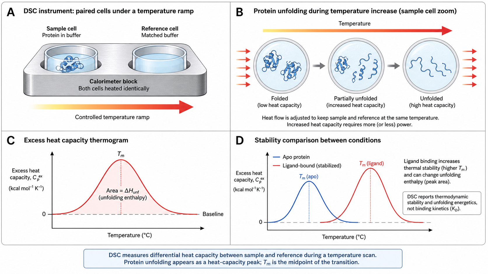
The experiment is conceptually simple: heat a protein solution and a matched buffer reference at the same rate. As the protein unfolds, it absorbs extra heat (the endothermic unfolding transition). The instrument measures the power difference needed to keep both cells at the same temperature. This power difference, converted to heat capacity, produces the characteristic DSC thermogram — a peaked curve where:
- Peak position = melting temperature Tm (midpoint of unfolding)
- Peak area = calorimetric enthalpy ΔHcal (total heat of unfolding)
- Peak shape = cooperativity and unfolding mechanism
Why DSC over DSF? DSF is faster and cheaper (20 min, plate reader), but DSC gives you thermodynamic quantities that DSF cannot: ΔHcal, ΔCp, and the ratio ΔHcal/ΔHvH which reveals whether unfolding is truly two-state. For regulatory filings, DSC is the expected method for thermal stability characterization of biotherapeutics.
Key Physics Concepts
📈 The DSC Thermogram
A DSC thermogram plots excess heat capacity Cpexcess (kJ/(mol·K)) vs. temperature (°C).
Tonset: Where the curve first departs from baseline. 5–15°C below Tm. More useful than Tm for aggregation-prone proteins.
Tm: Peak maximum — protein is 50% unfolded (two-state). Depends on intrinsic stability, pH, buffer, ionic strength, and excipients.
ΔHcal: Peak area = total heat absorbed. 200–800 kJ/mol for globular proteins (10–50 kDa).
ΔCp: Baseline shift between native and unfolded states. ~3–12 kJ/(mol·K) for typical small-to-medium globular proteins (scales with size, ~50–60 J·mol⁻¹·K⁻¹ per residue). Proportional to buried hydrophobic surface area.
🔀 Two-State vs. Non-Two-State
The ratio ΔHcal/ΔHvH is DSC's unique diagnostic for the unfolding mechanism.
Ratio ≈ 1.0: True two-state (N ⇌ U). Single cooperative unit. Small single-domain proteins.
Ratio > 1: Multiple domains unfolding independently. Broader peak = overlapping transitions. Antibodies, multi-domain proteins.
Ratio < 1: Intermolecular cooperativity — the cooperative unit is larger than one monomer (oligomeric unfolding). Note: aggregation/irreversibility distorts both quantities and is not cleanly diagnosed by this ratio.
ΔHvH = 4 R Tm² · Cpexcess(Tm) / ΔHcal — i.e. 4 R Tm² · (peak height / peak area), where the excess heat capacity at Tm is in kJ·mol⁻¹·K⁻¹ and ΔHcal in kJ·mol⁻¹, giving ΔHvH in kJ/mol.
📉 Gibbs-Helmholtz Stability Curve
DSC gives the full stability curve ΔG(T):
ΔG(T) = ΔHm(1 − T/Tm) − ΔCp[(Tm−T) + T·ln(T/Tm)]
ΔG = 0 at Tm — by definition (equal populations of N and U).
Tmax = temperature of maximum stability ≈ 10–30°C for most proteins.
Tcold = cold denaturation (hydrophobic effect weakens). Usually < 0°C.
ΔG(4°C) = practical storage stability — what actually matters for formulation.
Interactive Simulator
C_p^excess vs. Temperature
How DSC Works — Practical Guide
🧪 Experimental Setup
- Instrument: Power-compensation DSC (MicroCal PEAQ-DSC, VP-DSC) or heat-flux (TA Nano DSC). Power-compensation preferred for biomolecules.
- Sample: 0.1–2.0 mg/mL protein, 300–500 µL. Dialyze extensively — the reference buffer must be the dialysate.
- Degassing: Both sample and buffer under vacuum, 10–15 min at ~25°C. Dissolved gas → bubbles → noisy baselines.
- Scan rate: 1°C/min for equilibrium thermodynamics. Faster (2°C/min) for screening. If Tm shifts with rate → kinetically controlled.
- Temperature range: Start 10–20°C below expected Tonset, end 10–20°C above Tm. Typical: 20–100°C.
- Rescans: Always run a rescan (cool and reheat). Flat rescan = irreversible. Reproduced = thermodynamically reversible.
📊 Data Analysis
- Buffer subtraction: Subtract a buffer-buffer scan from the protein scan to remove instrument mismatch.
- Concentration normalization: Cp = (power − baseline) / (scan rate × moles of protein). Power in W divided by scan rate (K/s) and moles → Cp in J/(mol·K) (then convert to kJ/(mol·K)).
- Baseline: Progress baseline connecting pre- and post-transition. Choice affects ΔHcal by 5–15%.
- Integration: ∫Cpexcess dT = ΔHcal.
- ΔHvH: From peak shape: 4 R Tm² · Cpexcess(Tm) / ΔHcal = 4 R Tm² · (peak height in kJ·mol⁻¹·K⁻¹ / peak area in kJ·mol⁻¹).
- Multi-domain: Deconvolute into sum of independent two-state transitions. Each has its own Tm, ΔH.
- Reversibility: Compare scan 1 vs. rescan. ΔHrescan/ΔHfirst ≈ 1 = fully reversible.
Scan Rate & Reversibility
This is DSC's most misunderstood aspect.
Many protein transitions are irreversible — the unfolded protein aggregates before refolding. For irreversible transitions, the thermogram is NOT at equilibrium, and standard thermodynamic analysis (Gibbs-Helmholtz, ΔHcal/ΔHvH) is technically invalid.
Rescan test
Flat rescan = irreversible. Reproduced = reversible.
Scan rate dependence
Tm shifts higher at faster rates → kinetically controlled.
Peak asymmetry
Sharp leading edge + trailing tail → irreversible transition.
What you can still use: Tm (apparent — still useful for ranking), Tonset (more reproducible), ΔHcal (apparent). ΔHvH is meaningless for irreversible transitions — do not compute or report it.
Key Quantities from DSC
| Quantity | Symbol | Typical range | What it tells you |
|---|---|---|---|
| Melting temperature | Tm | 40–90°C | Thermal stability |
| Onset temperature | Tonset | Tm − 5 to −15°C | Start of unfolding |
| Calorimetric enthalpy | ΔHcal | 200–800 kJ/mol | Total heat of unfolding |
| van't Hoff enthalpy | ΔHvH | = ΔHcal if two-state | Cooperativity |
| Heat capacity change | ΔCp | ~3–12 kJ/(mol·K) | Hydrophobic exposure (scales with size) |
| Ratio | ΔHcal/ΔHvH | 1.0 = two-state | Unfolding mechanism |
Common Pitfalls
1. Buffer mismatch
Always use dialysate as reference — not fresh buffer. Even minor differences cause baseline artifacts.
2. Concentration too low
Below ~0.1 mg/mL signal is too weak for accurate ΔH. Use 0.5–1.0 mg/mL.
3. Concentration too high
Above ~2 mg/mL intermolecular aggregation during unfolding causes exothermic dips and irreproducible scans.
4. Not degassing
Dissolved gas forms bubbles during heating → spikes and noise. Always degas under vacuum.
5. Ignoring scan rate
If T_m shifts with scan rate, the transition is irreversible. Report "apparent T_m at X°C/min".
6. Wrong baseline
Progress baseline is most physical. Choice affects ΔH_cal by 5–15%. Be consistent within a study.
7. Confusing ΔH_cal with ΔH_vH
ΔH_cal = total measured heat. ΔH_vH = peak shape (two-state assumption). Only equal for true two-state.
8. Not running a rescan
Without a rescan, you cannot assess reversibility. Regulatory agencies expect this data.
Strengths & Limitations
✅ Strengths
- Direct thermodynamic measurement — no labels, dyes, or probes
- Tm, ΔHcal, ΔCp, ΔHvH from a single experiment
- ΔHcal/ΔHvH reveals unfolding mechanism
- Full stability curve ΔG(T) from Gibbs-Helmholtz
- Regulatory gold standard for thermal stability
- Multi-domain deconvolution resolves individual transitions
- Yields absolute thermodynamic quantities (ΔHcal directly from peak area), once the instrument's temperature and power calibration are in place
❌ Limitations
- Lower throughput than DSF (1–6 samples vs. 384/plate)
- Higher sample consumption: 300–500 µL at 0.5–1 mg/mL
- More expensive per sample ($50–200 vs. <$1 for DSF)
- Instrument cost: $100K–$300K
- Requires careful sample prep (dialysis, degassing)
- Irreversible transitions limit thermodynamic analysis
- Data analysis requires expertise (baseline, deconvolution)
When NOT to Use DSC
❌ High-throughput screening
500 buffer conditions? Use DSF (384-well, 20 min). Reserve DSC for the top 5–10 hits.
❌ Very dilute samples
Below ~0.1 mg/mL, signal-to-noise is too poor. Use DSF or nanoDSF (Prometheus, works at µg/mL).
❌ Intrinsically disordered proteins
IDPs have no defined folded state → no cooperative transition → no DSC peak.
❌ Membrane proteins in detergent
Detergent micelles have their own thermal transitions that overlap with protein transitions.
❌ When T_m is all you need
For rank-ordering formulations, DSF is equally accurate for T_m and much faster/cheaper.
❌ Kinetic stability
DSC measures thermodynamic stability. For kinetic stability, use isothermal denaturation by CD/fluorescence or HDX-MS.
DSC vs Related Techniques
🔥 DSC
- • Direct C_p measurement vs. T
- • T_m, ΔH_cal, ΔC_p, ΔH_vH
- • Full ΔG(T) stability curve
- • 0.3–0.5 mL at 0.5–1 mg/mL
- • 1–2 hours per sample
- • Best for: definitive characterization
🌡️ DSF/TSA
- • Fluorescence dye vs. T
- • T_m from inflection (no ΔH)
- • 5–25 µL, 384-well plate
- • 20 min
- • Best for: rapid screening
✨ nanoDSF
- • Intrinsic Trp fluorescence ratio
- • Label-free, very low concentration
- • 10 µL at 0.01–1 mg/mL
- • 15–30 min per capillary
- • Best for: label-free T_m
💿 CD Thermal Melt
- • Ellipticity (222 nm) vs. T
- • Secondary structure specific
- • 200–400 µL at 0.1–0.5 mg/mL
- • 30–90 min per scan
- • Best for: structure-specific stability
Publication Checklist
Experimental Details
- ☐ Instrument stated (manufacturer, model)
- ☐ Cell volume stated
- ☐ Protein concentration and MW stated
- ☐ Buffer composition stated
- ☐ Dialysis method stated (dialysate = reference)
- ☐ Degassing method stated
- ☐ Scan rate stated
- ☐ Temperature range stated
- ☐ Number of replicates
- ☐ Rescan result stated (reversible/irreversible)
Analysis & Results
- ☐ Buffer subtraction method stated
- ☐ Baseline type stated (progress, linear, cubic)
- ☐ T_m ± SD (°C) reported
- ☐ T_onset reported (if relevant)
- ☐ ΔH_cal ± SD (kJ/mol or kcal/mol) reported
- ☐ ΔH_vH reported (if two-state)
- ☐ ΔH_cal/ΔH_vH ratio with interpretation
- ☐ ΔC_p reported (if measurable)
- ☐ Deconvolution model stated (multi-domain)
- ☐ Scan rate noted if irreversible
- ☐ Thermogram figure (C_p vs. T) shown
- ☐ Software stated
🔬 DSC Instruments & Software
Instruments
- MicroCal PEAQ-DSC (Malvern) — current flagship; 130 µL cell, automated 6-sample magazine
- MicroCal VP-DSC (Malvern) — previous gen; 500 µL cell, manual; still widely used
- TA Instruments Nano DSC — heat-flux design; 300 µL cell; corrosive buffer compatible
- Setaram Micro DSC VII — high-sensitivity; 1 mL cells; for dilute samples
Software
- MicroCal PEAQ-DSC Software — integrated; baseline subtraction, two-state/non-two-state fitting
- Origin + DSC Add-on (OriginLab) — VP-DSC analysis; deconvolution
- NanoAnalyze (TA) — Nano DSC; multiple baseline types
- CpCalc — open-source DSC analysis
Have SPR or BLI data?
Upload your raw files and get an automated kinetic analysis in minutes. We support Biacore, Octet, and other major formats.
Upload & Analyze