🔬 Focal Molography

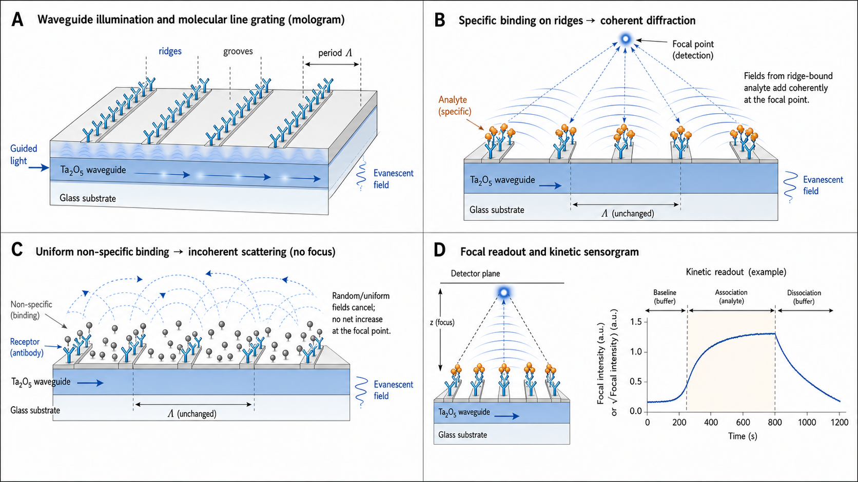
Focal molography is a label-free biosensing technique that detects molecular binding events through coherent diffraction from a nanoscale molecular grating — the "mologram." Receptor molecules are immobilized in a periodic pattern (pitch Λ ≈ 0.3–0.8 µm, typically ≈ 0.5 µm) on a waveguide surface. When analyte molecules bind specifically to the receptors, they create a periodic refractive index modulation in the evanescent field. Coherent light guided in the waveguide diffracts off this molecular grating and converges to focal spots both above and below the waveguide — much like a holographic lens. The lower focal spot (through the glass substrate) is the one measured, providing a stable optical path free from liquid flow perturbations. Its intensity is a direct readout of how much analyte has bound.

The defining advantage of focal molography is self-referencing: only molecules that bind in the periodic pattern (usually specifically to the immobilized receptors) contribute coherently to the diffracted focal spot. Spatially random non-specific adsorption has little Fourier weight at the grating wavevector K. Individual randomly bound molecules scatter with random phases and their fields add mostly incoherently. The resulting background intensity scales linearly with N_NSB, while the coherent focal spot from N periodically bound molecules scales as N² — a suppression ratio of ~N that grows with grating size. Bulk refractive index changes (buffer switches, temperature drift, DMSO in compound screens) affect all regions approximately equally and do not directly change the grating modulation. This gives focal molography strong first-order rejection of artifacts that plague refractometric methods like SPR.

🎯

Self-referencing

Random non-specific binding and uniform bulk RI shifts are strongly suppressed — periodically patterned binding dominates the focal spot. Incoherent scattering from random NSB scales as N (vs. N² for coherent signal), making it small for typical grating sizes.

🚫

Reduced referencing burden

Unlike SPR, a separate reference flow cell is usually not required for routine bulk-RI and uniform-NSB rejection. Spatial control molograms and image-registration drift correction are still used in practice for high-precision work.

🩸

Robust in crude matrices

Serum, plasma, cell lysate — random non-specific background mostly generates weak incoherent scattering rather than coherent diffraction signal.

📈

Label-free, real-time kinetics

Measure k_on, k_off, K_D in real time, like SPR — but without the referencing headaches.

📐

Quadratic signal scaling

Focal intensity ∝ (bound mass)² — because electric fields from each specifically bound molecule add coherently (in phase), amplitude ∝ N and intensity ∝ N². Signal grows faster than linear at high coverage.

Key Physics Concepts

🔬 The Molecular Grating & Focal Spot

Receptors patterned in a periodic structure (pitch Λ ≈ 0.3–0.8 µm, typically ≈ 0.5 µm) on a waveguide surface
Waveguide: Ta₂O₅ on glass, ~145 nm thick, n_wg ≈ 2.1 (λ = 632.8 nm)
He-Ne laser (λ₀ = 632.8 nm; commercial MACS Matchmaker uses 785 nm) excites a guided TE₀ mode with n_eff ≈ 1.814
Grating diffracts light at angle θ: sin(θ) = (n_eff − λ₀/Λ) / n_clad
Curved grating lines (holographic lens) → focal spots above and below the waveguide. The lower focus (substrate side, f ≈ 900 µm below) is measured — stable optical path through glass
Typical mologram: D ≈ 400 µm, f ≈ 900 µm (NA ≈ 0.33) → Airy-disk focal spot ~1–2 µm

📐 Quadratic Signal — I ∝ (Γ)²

Diffracted field amplitude: E_diff ∝ Δn_mod
Focal spot intensity: I_focal ∝ (Γ_specific)²
At 1% coverage: FM gives 0.01% of max signal vs. SPR's 1% → FM is 100× weaker at low Γ
At saturation: FM and SPR both at maximum — but FM is free of non-specific background
√I_focal ∝ Γ linearizes the response — always plot √I for kinetic analysis

🛡️ Self-Referencing & Background Immunity

Bulk RI: Uniform n_clad change → no Δn_mod change → I_focal unaffected. SPR: ~1000 RU from 10⁻³ RIU
Non-specific adsorption: Random fouling is spatially uniform → no periodic modulation change → only weak incoherent scattering (∝ N, negligible vs. coherent signal ∝ N²)
Temperature drift: Uniform thermal RI shift → preserved modulation contrast. SPR requires ±0.01°C control
Separate reference flow cell and buffer-blank subtraction usually not required — though spatial control molograms and image-registration drift correction remain best practice

Interactive Simulator

Grating pitchnm500 nm

Laser wavelengthnm660 nm

n_effguided mode1.78

Mologram diameterµm200 µm

Focal lengthmm1.0 mm

Outcoupling angle

20.2°

Focal spot diameter

6.1 µm

NA (effective)

0.132

Grating lines

400

Angular peak width

151.5 mdeg

Allowed Λ range

212–1467 nm

How Focal Molography Works — Practical Guide

🔬 Experimental Setup

Waveguide chip: Ta₂O₅ on glass (~150 nm), with pre-patterned molecular grating defined during chip fabrication
Mologram fabrication: Receptors immobilized at grating positions via interferometric photopatterning of a reactive surface layer. Typical: ~200 µm diameter, pitch ~500 nm
Light source: Coherent laser (632.8 nm He-Ne in the Frutiger 2019 research demonstrator; 785 nm laser diode in the commercial MACS Matchmaker), coupled into the waveguide. Coherent illumination of the mologram region
Detection: Camera (CCD/CMOS) positioned below the chip, imaging through the glass substrate. The lower focal spot (f ≈ 900 µm below the waveguide) is measured — stable optical path through glass, free from liquid flow perturbations. Signal = integrated intensity of focal spot
Fluidics: Flow cell over chip surface. Inject analyte → association → wash → dissociation
Readout: Focal spot intensity recorded in real time. Sensorgram: √I vs. time (linearized)

📊 Data Analysis

Image focal spot: Define ROI around the focal spot. Integrate pixel intensity → I_focal(t)
Linearize: Compute √I_focal(t) → signal proportional to coherent bound mass
Baseline: √I during buffer flow = baseline
Association: Fit to 1:1 Langmuir: √I(t) = √I_eq × (1 − exp(−k_obs × t))
Dissociation: Fit to single exponential: √I(t) = √I(t₀) × exp(−k_off × (t − t₀))
K_D: Kinetic (k_off/k_on) or steady-state √I_eq vs. [analyte]

Focal Molography vs SPR — What Changes

Same measurement goal (binding kinetics). Fundamentally different physics.

	Focal Molography	SPR
What's measured	Diffracted focal spot intensity (lower focus, through substrate) from molecular grating	Resonance angle shift from total surface RI change
Signal source	Coherently patterned (specific) binding dominates (∝ N²); incoherent NSB background (∝ N) is negligible	All mass at surface (specific + non-specific + bulk)
Signal scaling	I ∝ Γ² (quadratic); √I ∝ Γ (linear after transform)	Signal ∝ Γ (inherently linear)
Bulk RI	Strong first-order rejection	~130 deg/RIU — must be reference-subtracted
Non-specific	Small if random; correlated NSB can leak into signal	Adds directly to signal
Reference needed?	Usually no separate channel (self-referencing)	Yes (channel + buffer blank)
Sensitivity at low Γ	Lower (quadratic penalty)	Higher (linear, optimized instrumentation)
Best for	Crude matrices, compound screens	Detailed kinetics in clean buffers

Signal Scaling — Always Plot √I

Always plot √I_focal, not I_focal, for kinetic analysis.

I_focal ∝ Γ² means the raw sensorgram is nonlinear. A 1:1 Langmuir association looks like a compressed exponential in I, making fitting unreliable
√I_focal ∝ Γ linearizes the response — association looks like the familiar (1 − exp(−k_obs t)) curve
Standard kinetic fitting equations (1:1 Langmuir, mass transport, heterogeneous ligand) can be applied to the √I sensorgram, ideally with weighting because noise is heteroscedastic after the transform
Noise propagation: σ(√I) = σ(I) / (2√I) — at low signal, noise in √I is amplified

Key Quantities

Quantity	Symbol	Typical range	What it tells you
Grating pitch	Λ	0.3–0.8 µm	Determines outcoupling angle
Effective index	n_eff	1.6–1.9	Guided mode property
Focal spot intensity	I_focal	arbitrary	Raw signal (∝ Γ²)
√I signal	√I_focal	arbitrary	Linearized signal (∝ Γ_specific)
Coherent bound mass	Γ_coherent	0–5 ng/mm²	Specifically bound mass in grating
Grating modulation	Δn_mod	10⁻⁵ – 10⁻³ RIU	RI contrast of molecular grating
Dissociation constant	K_D	pM – µM	Binding affinity
Outcoupling angle	θ	5–60°	Where diffracted light exits
Focal spot diameter	d_spot	3–20 µm	Determined by NA of focusing grating
Mologram diameter	D	100–500 µm	Size of the grating element

Common Pitfalls

Analyzing raw I instead of √I

Raw I_focal is quadratic in Γ. Fitting 1:1 kinetics to I gives wrong k_on, k_off, K_D. Always linearize with √I before kinetic fitting.

Expecting SPR-like sensitivity at low analyte

Quadratic scaling: FM signal at 1% coverage is only 0.01% of saturation (vs. 1% for SPR). For very weak signals, FM has intrinsically lower SNR.

Damaged or contaminated grating

Physical damage or non-uniform receptor deactivation reduces diffraction efficiency globally — unlike SPR where defects cause local artifacts.

Grating pitch mismatch

Using a chip designed for one wavelength with a different laser gives no outcoupled signal. Verify λ, n_eff, and Λ are compatible.

Ignoring the duty cycle

Modulation efficiency depends on η. At η = 0 or η = 1, there is no modulation → no diffraction. Optimal η = 0.5. Poor patterning pushes η away from optimal.

Confusing signal vs. binding suppression

FM suppresses the signal from non-specific binding — it does NOT prevent non-specific binding. High NSB can still block receptor sites.

Camera saturation or dark current

At high binding, I_focal can saturate the camera. At very low binding, dark current dominates. Adjust exposure time accordingly.

Stray light at the focal plane

Scattered light from waveguide defects or dust creates background at the focal spot position. Dark-background imaging and spatial filtering are essential.

Strengths & Limitations

Strengths

Intrinsic self-referencing: often no separate reference channel needed (random NSB produces weak incoherent background ∝ N vs. coherent signal ∝ N²)
Works in crude matrices: serum, plasma, lysate — with strongly reduced solvent/background correction burden
Real-time, label-free kinetics (k_on, k_off, K_D)
Strong endpoint signals (quadratic scaling at high coverage)
Multiple molograms per chip → parallel measurements
No dextran matrix needed — flat waveguide surface

Limitations

Lower sensitivity at very low analyte (quadratic penalty at low Γ)
Requires pre-patterned waveguide chips — more fabrication complexity
Chip reuse depends on surface chemistry — DNA-based commercial chips can be highly regenerable, but regeneration must preserve the patterned affinity modulation and capture integrity
Fewer commercial instruments than SPR
Small molecule detection (< 300 Da) is challenging
√I linearization introduces noise amplification at low signal
Grating quality directly impacts signal quality

When NOT to Use Focal Molography

Fragment screening (< 300 Da)

Very small RI change per molecule + quadratic scaling → signal may be undetectable. Use SPR with enhanced sensitivity or TSA.

Detailed kinetics in clean buffers

If your matrix is clean (no NSB, no DMSO), SPR offers superior per-molecule sensitivity and a more mature ecosystem.

Very low-density analytes

Binding < 0.1 ng/mm²: quadratic signal scaling makes FM signal negligible. SPR's linear scaling gives better sensitivity.

Ultra-high throughput (> 10k compounds)

FM throughput depends on chip fabrication and fluidic cycles. For ultra-HTS, plate-based methods may be more practical.

Membrane protein kinetics

Reconstitution or membrane-on-chip complicates grating patterning. SPR with L1 or HPA chips is more established.

Single-molecule detection

FM measures ensemble diffraction from a grating — cannot resolve individual binding events. Use nanopore sensing or smFRET.

Technique Comparison

	🔬 Focal Molography	📡 SPR	📸 SPRi	🌊 FIDA
Sensor	Waveguide + molecular grating	Gold film, prism coupling	Gold film, array, camera	Capillary, fluorescence
Readout	Coherent diffraction (specific binding dominates; NSB suppressed by N²/N ratio)	Total RI change (all mass)	Total RI change (per spot)	Taylor dispersion
Referencing	Self-referencing (no ref needed; coherent signal ≫ incoherent background)	Ref channel essential	Array referencing (spatial)	In-solution (no surface)
Signal	I ∝ Γ² (use √I)	∝ Γ (linear)	ΔR ∝ Γ (linear)	σ_t ∝ √R_h
Label	Label-free	Label-free	Label-free	Fluorescent
Matrices	Serum, DMSO, lysate	Clean buffer preferred	Clean buffer preferred	Serum, lysate
Output	k_on, k_off, K_D	k_on, k_off, K_D	k_on, k_off, K_D	K_D + R_h
Best for	Crude matrix kinetics	Detailed kinetics	Throughput screening	In-solution K_D

Publication Checklist

🔬 Experimental

☐ Instrument and chip type (waveguide material, thickness, grating pitch)
☐ Mologram dimensions (diameter, number per chip)
☐ Receptor identity and immobilization chemistry
☐ Grating patterning method (e.g. interferometric photopatterning of reactive surface layer)
☐ Analyte identity and concentration range
☐ Buffer composition (especially if serum, DMSO, complex matrix)
☐ Flow rate and temperature
☐ Laser wavelength
☐ Camera specifications (exposure, frame rate)

📊 Analysis

☐ √I transformation stated and justified
☐ Baseline subtraction method described
☐ Kinetic fitting model stated (1:1 Langmuir, etc.)
☐ k_on, k_off, K_D reported ± SD or CI
☐ Goodness of fit (χ², residuals) shown
☐ Sensorgram shown (√I vs. time)
☐ Controls: blank injection, non-specific control
☐ Comparison with SPR or orthogonal method if claiming K_D agreement

Instruments & Software

Instruments

lino Biotech AG: Commercial focal molography platform based on curved molecular gratings and focal spot detection through the substrate
Research instruments: Academic and precommercial setups based on Fattinger's concept using curved molecular gratings, laser diode illumination, microscope optics, and camera-based focal spot detection

Note: GCI is a refractometric biosensor and should not be conflated with focal molography. Focal molography detects coherent diffraction from a patterned affinity grating; GCI measures refractive-index-induced phase/amplitude changes in a waveguide grating sensor.

Software

Vendor-provided: Chip alignment, focal spot detection, √I sensorgram extraction, kinetic fitting (1:1, mass transport)
Custom analysis: Python/MATLAB for advanced analysis (multi-analyte, heterogeneous binding, custom grating models)

Have SPR or BLI data?

Upload your raw files and get an automated kinetic analysis in minutes. We support Biacore, Octet, and other major formats.

Upload & Analyze