🌀 Fluorescence Polarization / Anisotropy (FP/FA)

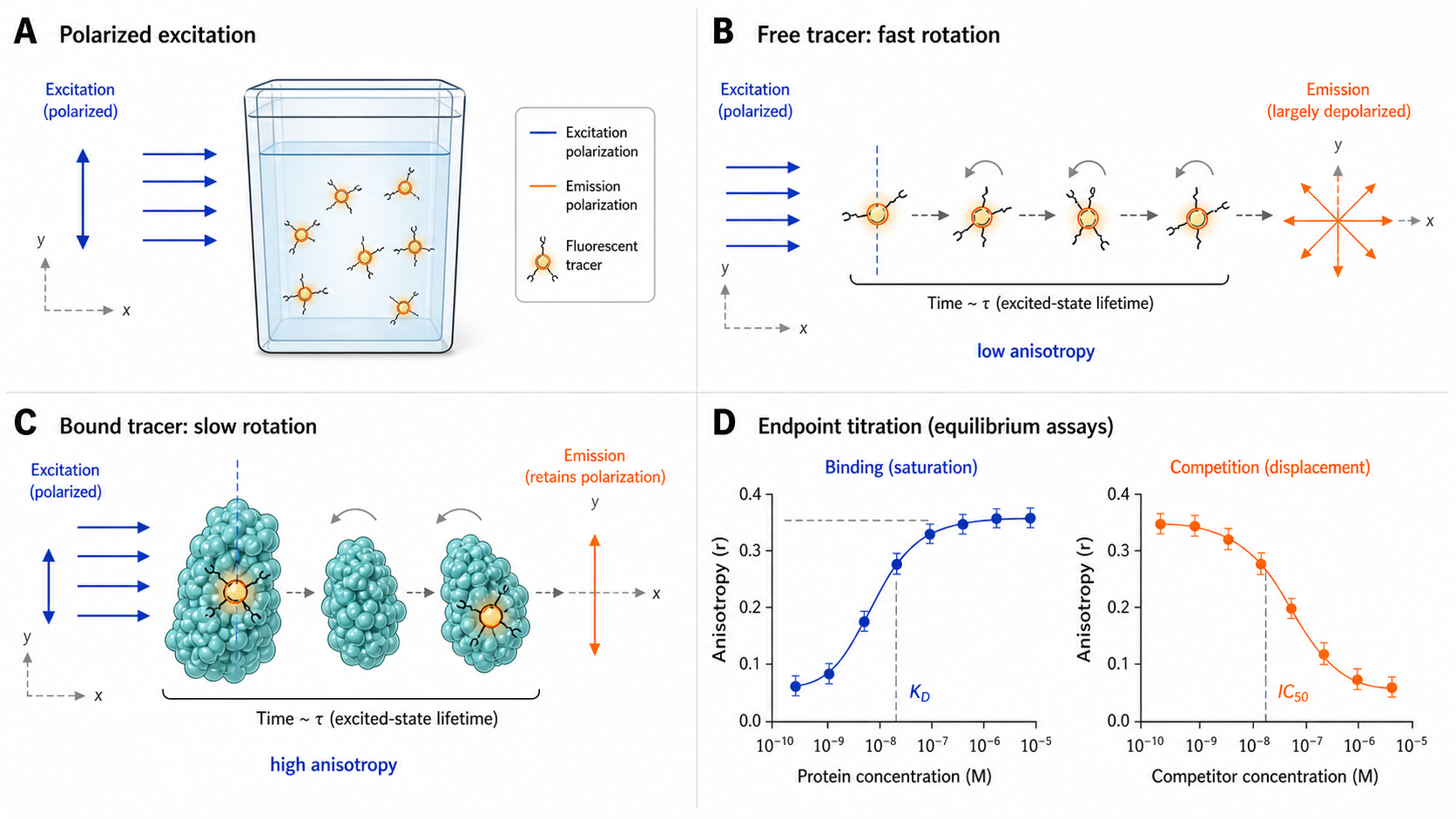
Figure 1 schematic explaining fluorescence polarization and anisotropy: polarized excitation, fast rotation of free tracer, slow rotation of protein-bound tracer, polarization readout, and binding curve analysis

Fluorescence polarization measures molecular rotation. When you excite a fluorophore with polarized light, the emitted light remains polarized only if the molecule hasn't tumbled during the fluorescence lifetime. A small, free tracer tumbles fast → low polarization. The same tracer bound to a large protein complex tumbles slowly → high polarization. Plot polarization vs. ligand concentration → sigmoidal binding curve → K_D. In drug screening, the most common format is competition FP, where a labeled tracer is pre-bound to the target and unlabeled compounds compete for the binding site — yielding K_i values for entire compound libraries.

FP is the workhorse of high-throughput screening (HTS) in drug discovery. Mix-and-read, no wash steps, no separation, no immobilization, compatible with 384- and 1536-well plates. It's been a pharma staple since the 1990s for good reason: it's simple, robust, and scalable. While this page uses "protein" as the default binding partner for readability, FP works for any macromolecule — DNA, RNA, lipid vesicles, carbohydrates — as long as the MW ratio is sufficient.

FP measures equilibrium K_D (like MST and ITC) — it does not give kinetic rate constants (k_a, k_d). For kinetics, use SPR or BLI. Unlike MST, FP requires a fluorescent tracer — either a fluorescently labeled ligand or a naturally fluorescent compound. The key constraint: the molecular weight ratio between the bound complex and the free tracer (MW_complex / MW_tracer) must be large enough to produce a measurable change in rotational correlation time — typically at least 5× in MW (conservative assays use 10×).

Key Physics Concepts

💡

Polarized Excitation & Emission

When plane-polarized light excites a fluorophore, only molecules whose absorption transition dipole is aligned with the electric field vector absorb efficiently — photoselection. If the molecule doesn't rotate before emitting, the emission retains its polarization. If it rotates during the fluorescence lifetime τ, the emission is depolarized.

📐

Polarization (mP) and Anisotropy (r)

Two related observables from the same measurement:

P = (I‖ − I⊥) / (I‖ + I⊥)

mP = 1000 × P

r = (I‖ − I⊥) / (I‖ + 2·I⊥)

r = 2P / (3 − P)

Anisotropy adds linearly for mixtures: r_obs = f_bound·r_bound + (1 − f_bound)·r_free. Polarization does not — always fit in r, not mP.

🔄

The Perrin Equation

r = r₀ / (1 + τ/φ)

r₀ = limiting anisotropy (≤ 0.4), τ = fluorescence lifetime (ns), φ = rotational correlation time (ns). Rule of thumb: φ (ns) ≈ MW (kDa) × 0.4 at 20°C in water. When τ ≈ φ: maximum sensitivity to size changes.

Interactive FP Simulator

Explore the physics of fluorescence polarization through interactive simulations.

Parameters

Binding partner MW100 kDa

Tracer: 0.5 kDa fluorescein-labeled ligand (τ = 4 ns, r₀ = 0.4)

φ (free tracer)0.20 ns

φ (bound complex)40.2 ns

r (free)0.019

r (bound)0.364

mP (free)28 mP

mP (bound)462 mP

Δr0.345

How FP Works — Measurement Principle

🔭 The Optical Setup

Excitation light passes through a polarizing filter (vertical), so only vertically polarized light hits the sample.
Emission is split by a polarizing beam splitter into I‖ (parallel) and I⊥ (perpendicular) channels.
Both intensities are measured simultaneously by two PMTs (T-format) or sequentially by rotating a polarizer (L-format). T-format is standard in plate readers.
r = (I_VV − G·I_VH) / (I_VV + 2G·I_VH), where G corrects for differential detector sensitivity.

⚖️ The G-Factor

The G-factor corrects for differential sensitivity of the detection system to horizontally vs. vertically polarized emission:

G = I_HV / I_HH

H excitation, V emission / H excitation, H emission

Without G-factor correction, systematic errors of 10–20% in r are common. Typical G values: 0.9–1.1. Modern plate readers auto-measure G with a free-dye sample — always calibrate.

Segmental Motion — The Hidden Assay Killer

The Perrin equation assumes the fluorophore is rigidly attached to the macromolecule. In reality, a dye connected via a flexible linker undergoes local rotation (segmental motion) independent of the overall protein tumbling. The correct steady-state expression (Lipari-Szabo model-free):

r = r₀ × [S² × φ_global/(φ_global + τ) + (1 − S²) × φ_eff/(φ_eff + τ)]

1/φ_eff = 1/φ_local + 1/φ_global — both motions contribute to depolarization

S² = order parameter (0–1)

S² = 1: rigid attachment → reduces to Perrin equation

S² → 0: dye wobbles freely → r dominated by fast φ_eff term

S² ≈ 0.7–0.9 for direct NHS lysine labeling (short linker)
S² ≈ 0.1–0.3 for dye on PEG₄ tether (flexible linker)

Example — 50 kDa protein:

φ_global = 20 ns, τ = 4 ns (FITC), flexible linker (φ_local = 0.3 ns, S² = 0.3)

Perrin prediction (rigid): r = 0.333

Lipari-Szabo (flexible): r = 0.119

Flexible linker cuts r_bound by 64%!

Fix: Keep the linker between dye and binding moiety short and rigid when possible. If r_bound is disappointingly low, try a different labeling position or shorter linker before changing fluorophores.

Assay Design — Key Experimental Parameters

FP Assay Design Checklist

Define the binding pair — What binds what? Which component gets labeled?
Choose the tracer — Label the smaller binding partner for maximum Δr.
Select the fluorophore — Match τ to the MW range (see Perrin Explorer). Fluorescein is the default.
Validate the tracer — Measure K_D of labeled tracer by direct saturation binding. Compare to unlabeled K_D.
Optimize [Tracer] — Use the lowest concentration that gives acceptable S/N. Rule: [T] < K_D/10 for accurate K_D.
Run saturation binding — Titrate protein vs. fixed [tracer] → determine K_D,tracer and confirm r_free and r_bound.
Set up competition — Fix [protein] and [tracer]; [P] should be near K_D,tracer for optimal sensitivity.
Equilibration time — Run a time course (0, 15, 30, 60, 90 min). Typical: 15–60 min at RT.
Controls — Tracer-only (baseline), tracer + saturating protein (max), DMSO blanks, positive control compound.
Plate layout — Randomize or interleave; avoid edge effects.

Tracer Concentration Regime

[T] vs K_D	Status	Consequence
[T] ≤ K_D/10	✅ Ideal	EC₅₀ ≈ K_D. Simple binding model valid.
K_D/10 < [T] < K_D	⚠️ Use quadratic	EC₅₀ shifts right. Use quadratic model; report [T].
[T] >> K_D	❌ Danger	Measuring stoichiometry. K_D is an upper limit. Reduce [T].

Protein Concentration in Competition

[Protein] vs K_D,tracer	Quality	Reason
[P] = K_D,tracer	✅ Optimal	50% of tracer is bound → maximum dynamic range for displacement
[P] = 3–5× K_D,tracer	⚠️ Acceptable	>75% tracer bound → still workable; need more competitor to displace
[P] >> K_D,tracer	❌ Problem	Nearly all tracer bound → competitors need extreme concentrations → lose sensitivity to weak binders

Assay Quality: Z′ Factor

Z′ = 1 − (3σ_pos + 3σ_neg) / |µ_pos − µ_neg|

Z′	Quality
> 0.5	✅ Excellent — suitable for HTS
0.2 – 0.5	⚠️ Marginal — optimize before screening
< 0.2	❌ Unacceptable — redesign the assay

Fluorophore Selection Guide

🟢

Fluorescein (FITC)

λ_ex/λ_em: 494/521 nm · τ ≈ 4.0 ns

✓ Universal, cheap, well-characterized

✗ pH-sensitive (pKa ≈ 6.4) — use buffer pH ≥ 7.5 for stable FP; photobleaches

Best for: small molecule tracers (0.3–2 kDa) binding to proteins 10–500 kDa

🟠

TAMRA

λ_ex/λ_em: 555/580 nm · τ ≈ 4.2 ns

✓ pH-insensitive, photostable, red-shifted

✗ More expensive, hydrophobic

Best for: assays where fluorescein gives problems; peptide tracers

🟢

Alexa Fluor 488

λ_ex/λ_em: 495/519 nm · τ ≈ 4.1 ns

✓ Brighter & more stable than FITC; pH-insensitive

✗ More expensive

Best for: high-quality assays where stability matters

💚

BODIPY-FL

λ_ex/λ_em: 503/512 nm · τ ≈ 5.7 ns

✓ Narrow emission, high QY, pH-insensitive

✗ Hydrophobic — can cause non-specific binding

Best for: when spectral purity is important

💜

Dansyl

λ_ex/λ_em: 335/518 nm · τ ≈ 10–15 ns

✓ Longest conventional τ — ideal for peptide tracers (2–20 kDa)

✗ UV excitation; τ is environment-dependent (changes upon binding!)

⚠ Verify τ stability before committing to quantitative K_D extraction

Best for: peptide/small protein tracers binding large complexes

🔴

Cy5 / Alexa Fluor 647

λ_ex/λ_em: 649/670 nm · τ ≈ 1.0 ns

✓ Far-red, minimal autofluorescence

✗ Short τ compresses window for peptide-sized tracers

Best for: small-molecule tracers in autofluorescent samples

Fluorophore Decision Tree

Is your tracer a small molecule (<2 kDa)?

→ YES: Fluorescein or Alexa 488 (τ ≈ 4 ns = ideal)

→ NO: Is it a peptide (2–20 kDa)?

→ YES: TAMRA, Alexa 488, or dansyl (longer τ for bigger peptides)

→ NO: Is it a protein?

→ Is the binding partner >5× larger?

→ YES: Any dye works; fluorescein is cheapest

→ NO: Use long-lifetime dyes (pyrene) or TR-FRET

Is autofluorescence a problem (cell lysates, serum)?

→ YES: Alexa 647 / Cy5 or TR-FP (time-gated)

Are you doing HTS (>10,000 wells)?

→ YES: Fluorescein (cheapest, well-validated)

Common FP Assay Formats

📈

Saturation Binding

Fix [tracer], titrate [protein]. Anisotropy increases as tracer binds → saturation curve → K_D,tracer, r_free, r_bound. Always run this first to characterize the tracer before competition assays.

⚔️

Competition / Displacement

Fix [protein] + [tracer] at equilibrium; titrate unlabeled competitor. Anisotropy decreases → IC₅₀ → K_i via Cheng-Prusoff. Most common format in drug discovery — screen compound libraries.

⚡

Enzyme-Linked FP

Fluorescently labeled substrate; enzyme cleaves it → smaller product → anisotropy drops. Inhibitors prevent cleavage → high anisotropy. Yields IC₅₀ of inhibitor. Used for protease, kinase, nuclease assays. Note: functional assay, not direct binding.

🔗

Ternary Complex (PROTACs)

Label one protein; add bifunctional compound + second protein. Ternary complex formation → MW increase → higher anisotropy. Hook effect: at high [compound], bell-shaped dose-response. EC₅₀ of rising phase reflects potency; hook concentration = binary saturation.

Data Analysis

Binding Models

Intensity weighting: Anisotropy is additive over intensity fractions. If quantum yield changes upon binding, use the intensity-weighted model. Always check total fluorescence intensity across the titration — if it changes >15–20%, use the intensity-weighted model or switch fluorophores.

Direct Saturation (simple)

r = r_free + (r_bound − r_free) × [P] / ([P] + K_D)

Valid when [T] << K_D

Saturation (quadratic — with tracer depletion)

[PT] = ½{([P]_t + [T]_t + K_D) − √(…² − 4[P]_t[T]_t)}
r = r_free + (r_bound − r_free) × [PT] / [T]_t

Competition (Cheng-Prusoff approximation)

K_i = IC₅₀ / (1 + [T]_free / K_D,tracer)

[T]_free ≈ [T]_total when fraction bound is small

Important: r_top ≠ r_bound

In competition, r_top (starting anisotropy) depends on fraction bound at the chosen [P] and K_D,tracer. At [P] ≈ K_D,tracer, only ~50% is bound → r_top ≈ (r_free + r_bound)/2. Use measured control values, not theoretical ones.

Common Pitfalls in FP Data Analysis

Confusing EC₅₀ with K_D

EC₅₀ = K_D only when [tracer] << K_D. Otherwise EC₅₀ > K_D. Always report which one you measured.

Fitting in mP instead of r

Polarization does not add linearly for mixtures. Best practice: convert to r, fit, convert back to mP for display.

Neglecting the G-factor

Without instrument correction, r is systematically wrong. Run a free-dye calibration every session.

Inner filter effect

High [fluorophore] or compound absorbs excitation/emission light. Keep OD < 0.1 at both λ_ex and λ_em.

Compound autofluorescence / quenching

Compounds may fluoresce (especially green channel!) or quench the tracer. Run a tracer-only + compound control.

Temperature sensitivity

Viscosity drops ~2–3% per °C → φ decreases → r decreases. A 5°C drift across a plate causes systematic error.

Aggregation / promiscuous binding

Colloidal aggregates sequester protein → apparent displacement. Add 0.01–0.05% Triton X-100 to discriminate.

DMSO mismatch

DMSO increases viscosity → r increases. Keep DMSO constant across all wells including controls.

Light scattering at high [protein]

At high protein (>10 µM), Rayleigh scattering increases apparent polarization. Add long-pass emission filter.

10.

PMT saturation

At very high fluorescence, nonlinear detector response distorts the I‖/I⊥ ratio. Keep counts in the linear range.

11.

Viscosity modulation — deliberate and accidental

Adding glycerol or sucrose slows tumbling and increases r_bound — a useful lever for assays where Δr is too small. The flip side: viscosity changes with temperature, freeze-thaw history, and buffer batch; even 5% glycerol variation shifts r. Keep buffer composition identical across all wells, including blanks and controls.

Strengths & Limitations

✅ Strengths	❌ Limitations
Homogeneous — mix-and-read, no wash steps	Requires fluorescent tracer (labeled or intrinsic)
HTS-compatible: 384-well and 1536-well	MW ratio must be ≥5× for adequate Δr
Equilibrium K_D in solution	Cannot distinguish competitive vs. allosteric binding
Fast — minutes to equilibrium, seconds to read	Fluorescence interference: autofluorescent/colored compounds
Very low sample: µL volumes, nM concentrations	No kinetic information (k_a, k_d)
Simple instrumentation (any FP plate reader)	Inner filter effect at high concentrations
No immobilization — true solution measurement	Temperature-sensitive (viscosity changes affect r)
Robust — validated protocols for hundreds of targets	Protein–protein interactions (both large) give minimal Δr
Competition format gives K_i for unlabeled compounds	Aggregating/promiscuous compounds give false positives
TR-FP variants reduce background for crude samples	Cheng-Prusoff K_i is approximate; exact solutions are complex

Time-Resolved Fluorescence Polarization (TR-FP)

TR-FP uses a time gate to reject short-lived background before measuring FP. The canonical implementations use long-lifetime organic fluorophores — Ru(II) polypyridyl complexes (τ ≈ 100–1000 ns), pyrene (τ ≈ 100–400 ns in deoxygenated solvent), acridone, dansyl — or fluorescence-lifetime gating on conventional dyes. After pulsed excitation, wait long enough for autofluorescence (ns lifetime), scattered excitation, and plate background to decay before integrating emission.

Note on lanthanides: lanthanide chelates (Eu³⁺, Tb³⁺, τ ≈ 100–1000 µs) are sometimes loosely grouped under "TR-FP," but their f–f emission has a poorly defined emission dipole and near-zero intrinsic anisotropy (r₀ ≈ 0). They are the basis of TR-FRET assays (LanthaScreen, HTRF), not of practical TR-FP — even with a perfect time gate, there is no polarization signal to measure.

Common misconception: TR-FP does NOT extend the MW sensitivity range

Even at the long end of organic-dye lifetimes, τ has to be matched to φ for a measurable r. Hypothetically with a τ ≈ 500 µs lanthanide and a 500 kDa complex (φ ≈ 200 ns), τ/φ ≈ 2500 → r ≈ 0 — fully depolarized (and lanthanide r₀ is already ≈ 0). The time gate eliminates background; it does not shift the sensitive MW window. To extend that window you must change the fluorophore τ, not gate on it.

TR-FP excels at:

HTS in crude matrices (cell lysates, serum, conditioned media)
Colored compound libraries — autofluorescence gone after time gate
Higher Z′ values — reduced background variance

To extend FP to larger complexes, use:

Pyrene (τ ≈ 100–400 ns) → matches φ of 250–1000 kDa complexes
Acridone (τ ≈ 15–30 ns) → matches φ of 40–75 kDa complexes
Dansyl (τ ≈ 10–15 ns) → matches φ of 25–40 kDa complexes

TR-FP vs TR-FRET: TR-FP measures polarization of donor emission only — same binding events as conventional FP, lower background. TR-FRET measures sensitized acceptor emission after energy transfer — proximity-based, requires labeling both partners, more common in HTS due to dual-wavelength specificity.

When NOT to Use FP

❌ When both binding partners are large

A 50 kDa protein binding a 60 kDa protein: MW changes from 50 → 110 kDa. With fluorescein (τ = 4 ns): r_free ≈ 0.333, r_bound ≈ 0.367, Δr = 0.034 — too small. Use SPR, MST, or ITC instead.

❌ When you need kinetics

FP is equilibrium only. No k_a, k_d, or residence time information. Use SPR or BLI for kinetics.

❌ When binding changes fluorophore properties

If binding quenches or enhances fluorescence >20%, the intensity-weighted average is unreliable. Check total fluorescence across the titration.

❌ When compound autofluorescence dominates

Some chemical libraries have significant green fluorescence. Screen in the red channel (TAMRA, Cy5) or use time-resolved FP.

❌ For fragment screening

Fragment K_D is typically 0.1–10 mM — requires mM concentrations, causing inner filter effects and solubility issues. Better: TSA/DSF, SPR, or ligand-observed NMR (STD, WaterLOGSY).

❌ When label-free is required

FP requires a fluorophore. If modification is not acceptable, use SPR, BLI, or MST label-free (UV detection of tryptophan).

FP for Drug Discovery

🔍 Primary Screening (HTS)

384/1536-well competition format
Screen 10,000–1,000,000 compounds at single concentration
Z′ > 0.5 required
Hits: Δr > 3σ below control mean
Cost: ~$0.05–0.20 per well (reagent cost)
Throughput: 50,000–100,000 data points/day/reader

✅ Hit Validation & Dose-Response

Confirm hits with 8–12 point dose-response (half-log dilution)
Determine IC₅₀ for each confirmed hit
Convert IC₅₀ → K_i with Cheng-Prusoff
Counter-screens: autofluorescence, aggregation (Triton test)
Orthogonal validation: SPR, MST, or ITC for top compounds

⚗️ SAR & Lead Optimization

16–24 analogs per plate, full dose-response each
Compare K_i values to guide medicinal chemistry
Monitor selectivity vs. off-target proteins in parallel
Feeds into biophysics cascade alongside SPR characterization

FP vs Other Techniques

🌀 FP/FA

Equilibrium K_D (via K_i in competition)
Requires fluorescent tracer
HTS-compatible (384/1536-well)
µL volumes, nM concentrations
Fastest readout (seconds per well)
MW ratio constraint
No kinetics, no thermodynamics

🔬 MST

Equilibrium K_D
Requires fluorescent label (or label-free UV)
16-point capillary format
No MW constraint (works for any size)
Works in crude lysates
Lower throughput than FP for HTS
No kinetics, no thermodynamics

✨ SPR

Kinetics (k_a, k_d, K_D)
Label-free
Requires surface immobilization
Gold standard for drug–target kinetics
Higher throughput with multi-channel systems
Regulatory acceptance for biosimilars
Expensive instruments

Key message: FP excels at high-throughput equilibrium screening. MST excels at solution-phase characterization without MW constraints. SPR excels at kinetic characterization. They are complementary, not competitive.

Publication Checklist

Experimental Design

☐Tracer K_D determined by direct saturation binding
☐[Tracer] stated and < K_D/10 (or justified)
☐[Protein] in competition ≈ K_D,tracer (or justified)
☐G-factor measured and applied
☐Temperature controlled and reported
☐Equilibration time validated (time course)
☐DMSO concentration matched across all wells

Data Quality

☐Z′ > 0.5 for screening data
☐Δr (or ΔmP) reported
☐Both baselines (free and bound) well-defined
☐Counter-screen for compound interference
☐≥ 3 independent replicates for K_D/K_i values
☐Total fluorescence intensity checked (no quenching)
☐r_bound compared to Perrin prediction — segmental motion noted if low

Reporting

☐K_D or K_i ± CI (not just IC₅₀)
☐Binding model specified (Hill, simple, quadratic)
☐Cheng-Prusoff correction applied and stated
☐Fluorophore, wavelengths, and reader model reported
☐Raw anisotropy or mP data shown (not just normalized)
☐Orthogonal validation for key compounds (SPR, ITC, MST)

Instruments using Fluorescence Polarization

BMG LABTECH PHERAstar FSX — gold standard FP plate reader, dual PMT (T-format), TR-FP module
BMG LABTECH CLARIOstar Plus — excellent FP module with LVF monochromators
Tecan Spark — multimode reader with FP capability
Tecan Infinite M1000 Pro — quad-monochromator, good FP performance
PerkinElmer EnVision — HTS workhorse, TRF and FP modules, TR-FP
Molecular Devices SpectraMax — FP-capable multimode readers
BioTek Synergy Neo2 — dual PMT, good FP with temperature control

Have SPR or BLI data?

Upload your raw files and get an automated kinetic analysis in minutes. We support Biacore, Octet, and other major formats.

Upload & Analyze