⚡ Förster Resonance Energy Transfer (FRET)
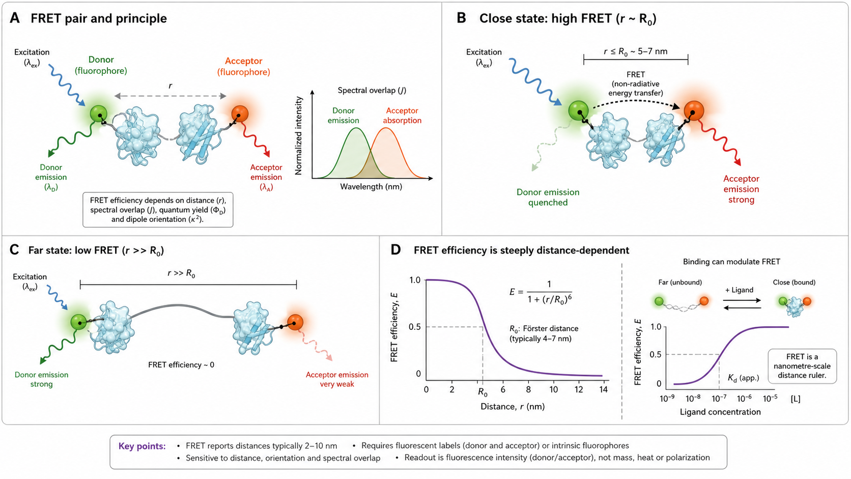
FRET is the molecular ruler of biophysics. When a donor fluorophore absorbs light, it can transfer energy non-radiatively to a nearby acceptor fluorophore — but only if they're close enough (typically 1–10 nm). The efficiency of this energy transfer drops as the sixth power of distance, making FRET exquisitely sensitive to nanometer-scale changes: protein conformational changes, binding events, membrane dynamics, even the precise distance between two labeled residues.
In practice, FRET experiments fall into two regimes crossed with two donor chemistries:
- Ensemble FRET (prompt fluorophore donors) — bulk measurement of average FRET efficiency across many molecules. Simple, fast, works on a plate reader. Used for binding assays and conformational screening.
- TR-FRET (time-resolved FRET) — also an ensemble technique, but uses lanthanide donors (Eu³⁺, Tb³⁺) with millisecond lifetimes instead of prompt fluorophores. Time-gating eliminates background fluorescence → excellent for high-throughput drug screening (HTRF, LANCE). The dominant homogeneous assay format in pharma.
- smFRET (single-molecule FRET) — measures FRET efficiency one molecule at a time. Reveals conformational distributions, dynamics, and rare states invisible to ensemble measurements. The gold standard for structural dynamics.
- Homo-FRET — FRET between two identical fluorophores, detected as a decrease in fluorescence anisotropy rather than sensitized emission. Widely used for receptor oligomerisation studies in live cells.
What FRET doesn't do easily: FRET measures distances, not affinities. You can detect binding (FRET appears when donor and acceptor are brought together), but extracting KD requires careful control of labeling stoichiometry and accounting for incomplete labeling. For KD, use SPR, MST, ITC, or FP. FRET excels at answering "where" and "how far" rather than "how tight."
Key Physics Concepts
The Förster Equation — FRET Efficiency
FRET efficiency E is the fraction of donor excited-state energy transferred to the acceptor:
E = R₀⁶ / (R₀⁶ + r⁶) = 1 / (1 + (r/R₀)⁶)- At r = R₀: E = 0.5 (50% transfer)
- At r = 0.5 × R₀: E = 0.984 (near-complete)
- At r = 1.5 × R₀: E = 0.081 (mostly gone)
- At r = 2 × R₀: E = 0.015 (negligible)
Practical FRET window: ~0.5 R₀ to ~1.5 R₀. Outside this range, E is either saturated or undetectable.
Measuring E experimentally:
Method 1 — Donor quenching: E = 1 − FDA/FD
Method 2 — Sensitized emission (proximity ratio): Eapp = IA / (IA + ID). Requires corrections for crosstalk, direct excitation, and γ factor.
Method 3 — Fluorescence lifetime: E = 1 − τDA/τD. Most rigorous — independent of concentration and labeling efficiency.
R₀ — The Förster Radius
R₀ defines the sensitivity range of a FRET pair. At r = R₀, E = 50%.
R₀⁶ = (9 × QD × κ² × ln10) / (128π⁵ × n⁴ × NA) × J(λ)QD = donor quantum yield; κ² = orientation factor (≈2/3); n = refractive index; J(λ) = spectral overlap integral.
| Donor / Acceptor | R₀ (nm) |
|---|---|
| ECFP / EYFP | 4.9 |
| mTurquoise2 / mVenus | ~5.4 |
| Cy3 / Cy5 | 5.4 |
| Alexa 488 / Alexa 594 | 5.4 |
| ATTO 550 / ATTO 647N | 6.5 |
| Eu-cryptate / d2 | ~9 |
R₀ values vary ±0.5 nm depending on labeling environment and buffer. Always measure under your experimental conditions for quantitative distance work.
Spectral Overlap & κ²
Spectral overlap integral J(λ):
J(λ) = ∫ FD(λ) × εA(λ) × λ⁴ dλGreater overlap between donor emission and acceptor absorption → larger J(λ) → larger R₀ → FRET over longer distances.
Orientation factor κ²:
κ² = (cos θDA − 3 cos θD cos θA)²κ² ranges from 0 (perpendicular dipoles) to 4 (collinear, head-to-tail parallel dipoles); two parallel side-by-side dipoles give κ² = 1. When both fluorophores rotate freely on a timescale faster than the donor lifetime (dynamic averaging), κ² = 2/3.
Impact: Since R₀ ∝ κ²^(1/6), a 2× error in κ² changes R₀ by only ~12%. That is acceptable for binding assays. For rotationally restricted dyes, however, κ² can in principle range from 0 to 4 — worst-case uncertainty can give 30%+ distance error, which matters for structural biology.
Interactive FRET Simulator
Practical FRET window
The shaded region (0.5 R₀ to 1.5 R₀) is where E is sensitive to distance changes. Outside this range, E is either saturated or negligible.
How FRET Works — Detection Methods
🔬 Ensemble FRET (Plate Reader / Fluorometer)
- Excite at donor wavelength
- Measure donor emission (quenched) and/or acceptor emission (sensitized)
- Calculate E from donor quenching or sensitized emission ratios
Corrections required:
- Direct excitation of acceptor at donor wavelength
- Spectral bleedthrough of donor into acceptor channel
- Incomplete labeling (donor-only or acceptor-only molecules)
Simple, high throughput. Gives only population average.
⏱️ TR-FRET (Time-Resolved FRET)
- Donor: Eu³⁺ cryptate (τ ≈ 0.6–1 ms) or Tb³⁺ chelate (τ ≈ 1.5–3 ms)
- Excitation: UV flash (320–340 nm)
- Time gate: Wait 50–150 µs → all short-lived fluorescence decays → only long-lived sensitized emission remains
- Detection: Two channels — donor reference (620 nm Eu; Tb is read at 490 nm on HTRF or 545 nm on LANCE) and sensitized acceptor (665 nm d2/XL665)
- Ratiometric: HTRF ratio = (665 nm / 620 nm) × 10,000
Advantages: Background rejection (S/B 100–1000×), no wash steps, HTS-compatible (384/1536-well).
Commercial: HTRF (Revvity), LANCE (Revvity), LanthaScreen (Thermo Fisher).
🔬 smFRET (Single-Molecule FRET)
- Microscopy: TIRF or confocal
- Excitation: Laser at donor wavelength (e.g., 532 nm for Cy3)
- Detection: Split path with dichroic → donor camera + acceptor camera
- Analysis: E per molecule per time bin → FRET histograms or time traces
- ALEX/PIE: Identifies active FRET pairs vs. donor-only / acceptor-only
Reveals: Conformational distributions, transition rates, rare states.
Requires: pM concentrations, specialized microscope, oxygen scavenging system.
⏲️ FLIM-FRET (Fluorescence Lifetime Imaging)
- Principle: Maps donor lifetime pixel-by-pixel in a microscopy image — FRET shortens τD
- Detection: TCSPC (time-correlated single-photon counting) or frequency-domain FLIM
- E from lifetime: E = 1 − τDA/τD
- Advantages: Independent of fluorophore concentration and laser intensity; spatially resolved; no acceptor needed for donor-quenching readout
Gold standard for live-cell FRET imaging — avoids spectral bleedthrough and direct-excitation artifacts.
Instruments: PicoQuant LSM upgrade, Leica SP8 FALCON, Becker & Hickl TCSPC modules.
FRET Pair Selection Guide
Choosing the wrong FRET pair is the #1 cause of failed FRET experiments. Before ordering reagents, verify that R₀ matches the expected distance.
Selection Criteria
- R₀ must match expected distance. Use the simulator (Tab 1) to verify your pair's practical window (0.5–1.5 × R₀) covers the expected D-A distance.
- Spectral separation. Donor emission and acceptor emission peaks should be >50 nm apart to minimize bleedthrough.
- Donor quantum yield. Higher QD → larger R₀ → FRET over longer distances.
- Acceptor extinction coefficient. Higher εA → larger J(λ) → larger R₀.
- Photostability. Critical for smFRET. ATTO 550/ATTO 647N outperform Cy3/Cy5.
- Labeling chemistry. NHS esters (lysines), maleimides (cysteines), click chemistry (unnatural amino acids). Site-specific labeling crucial for smFRET.
- Cell permeability. For live-cell FRET: genetically encoded FPs (CFP/YFP) or SNAP/Halo-tag dyes.
Application → Recommended FRET Pairs
| Application | Donor | Acceptor | R₀ (nm) | Why |
|---|---|---|---|---|
| Live cell FRET | mTurquoise2 | mVenus | ~5.4 | Genetically encoded, modern preferred pair |
| In vitro binding | Alexa 488 | Alexa 594 | 5.4 | Photostable, well-characterized |
| smFRET (standard) | Cy3 | Cy5 | 5.4 | Canonical pair, extensive literature |
| smFRET (photostable) | ATTO 550 | ATTO 647N | 6.5 | Better photostability than Cy3/Cy5 |
| HTS / TR-FRET | Eu-cryptate | d2 (HTRF) | ~9 | Time-gating, homogeneous, ratiometric |
| DNA/RNA structure | Cy3 | Cy5 | 5.4 | Conjugated to modified nucleotides |
TR-FRET for Drug Discovery
TR-FRET is one of the two dominant HTS assay formats in the pharmaceutical industry (alongside FP). The HTRF platform (Revvity, formerly Cisbio) is the most widely used.
⚗️ How HTRF / LANCE Assays Work
- Label target protein with Eu-cryptate (donor) — typically via anti-tag antibody (anti-His, anti-GST, anti-Flag)
- Label binding partner/tracer with d2 or XL665 (acceptor) — directly or via streptavidin-d2 + biotinylated peptide
- Mix in 384- or 1536-well plate
- Flash lamp excitation at 320 nm → time gate 50–150 µs delay → detection at 665 nm (acceptor) and 620 nm (Eu reference)
- HTRF ratio = (665 nm / 620 nm) × 10,000
Competition format for screening: Pre-form Eu-target + d2-tracer complex → high ratio. Add compound → displaces tracer → ratio decreases → IC₅₀ from dose-response.
⚖️ TR-FRET vs FP for HTS
| Feature | TR-FRET | FP |
|---|---|---|
| Background rejection | ✅ Excellent | ⚠️ Moderate |
| Fluorescent compound interference | ✅ Low | ❌ High |
| Dynamic range | ✅ Large | ⚠️ Small |
| Protein size requirement | ✅ None | ⚠️ Must be large |
| 1536-well miniaturization | ✅ Standard | ⚠️ Possible |
| Cost per well | ⚠️ Higher | ✅ Lower |
| Assay development complexity | ⚠️ More complex | ✅ Simpler |
smFRET — Conformational Dynamics
What smFRET Reveals
- Conformational distributions: The full histogram shows what fraction is in each state
- Dynamics: Time traces show transitions in real time (ms–s)
- Rare states: 5% populations invisible to ensemble average
- Heterogeneity: Static vs. dynamic disorder
- Absolute distances: Convert E to r via R₀ and the Förster equation
Experimental Requirements
- pM–nM concentrations (single-molecule regime)
- Photostable dyes (ATTO 550/647N, Cy3B/ATTO 647N)
- Oxygen scavenging system (glucose/glucose oxidase/catalase or PCA/PCD)
- Triplet-state quencher (Trolox or COT)
- PEG-coated passivated glass surfaces (surface-immobilized smFRET)
- ALEX/PIE to identify active FRET pairs vs. donor-only / acceptor-only
- Software: SPARTAN, FRETBursts, DeepFRET, iSMS
Corrections Required
- γ factor: Different detection efficiencies and quantum yields. Ecorr = Eapp / (Eapp + γ(1 − Eapp))
- Direct excitation: Acceptor excited by donor laser → subtract using ALEX/PIE data
- Crosstalk (leakage): Donor emission in acceptor channel → subtract measured crosstalk fraction
- Background: Subtract dark counts and buffer fluorescence
Assay Design Considerations
For Ensemble / TR-FRET Binding Assays
- Choose FRET pair with R₀ matching expected complex geometry. Crystal structure or homology model → estimate D-A distance. If unknown, use TR-FRET (R₀ ~ 9 nm, forgiving window).
- Label donor and acceptor at defined positions. Anti-tag antibodies with pre-conjugated Eu/d2 are simplest for proteins.
- Titration: Titrate acceptor-labeled partner against fixed donor-labeled target → KD from sigmoidal fit.
- Controls: Donor-only, acceptor-only, and both labels + competitor (baseline FRET).
- Z′ factor for screening: Z′ = 1 − 3(σp + σn)/|µp − µn|. Aim for Z′ > 0.5.
For smFRET
- Site selection: Choose solvent-exposed residues that don't perturb function. Introduce single cysteines for maleimide labeling (engineer out native Cys).
- Stochastic labeling: When using two dyes with one protein, labeling is random → must filter for donor-acceptor pairs using ALEX.
- Verify labels don't perturb protein: Activity assay, CD spectrum, SEC-HPLC before and after labeling.
- Controls: DNA ruler with known FRET efficiency for microscope calibration.
Common Pitfalls
Choosing FRET pair without considering R₀ vs. expected distance
If r >> 1.5 R₀, you won't see any FRET. Check with the distance calculator (Tab 1) before starting. This is the most common reason FRET experiments fail.
Ignoring incomplete labeling
Apparent E_max is reduced by the product of labeling efficiencies (e.g., 0.6 × 0.6 = 0.36). For smFRET with equimolar D/A dyes, ~50% of doubly-labeled molecules have the correct D-A configuration. Incomplete labeling reduces assay window but doesn't bias K_D if labeled fractions are equal.
Direct excitation contamination
If the donor excitation wavelength also excites the acceptor, "FRET" signal includes non-FRET acceptor emission. Always measure acceptor-only control and subtract.
Photobleaching masquerading as FRET
Donor photobleaching reduces donor emission → looks like donor quenching by FRET. Acceptor photobleaching control: bleach the acceptor → if donor emission increases, FRET was real.
Assuming κ² = 2/3 without checking
Measure donor anisotropy: r < 0.2 confirms fast rotation and validates κ² ≈ 2/3. If r > 0.3, the fluorophore is rotationally constrained → κ² uncertainty increases → distance error increases.
Over-interpreting absolute distances from ensemble FRET
Ensemble E is the population-weighted average of individual FRET efficiencies. Because E depends non-linearly on r, <E> ≠ E(<r>). Especially problematic for IDPs or flexible linkers.
Hook effect in TR-FRET
At very high reagent concentrations, signal can decrease paradoxically. Always run full dose-response curves; never rely on single-concentration measurements.
Confusing FRET ratio with binding fraction
In TR-FRET, the HTRF ratio is proportional to binding but not equal to fraction bound — it depends on labeling efficiency, antibody valency, and assay geometry. Use standard curves or calibrate against orthogonal methods.
Attributing all FRET signal changes to distance
A change in apparent FRET efficiency can arise from changes in κ² (dye reorientation), Q_D (donor quantum yield shift due to local environment), or refractive index — not just a change in donor-acceptor distance. This is a classical pitfall in conformational FRET: apparent distance changes may really reflect κ² or environment effects. Always report donor anisotropy and, where possible, use lifetime-based FRET to separate distance from other variables.
Strengths & Limitations
| ✅ Strengths | ❌ Limitations |
|---|---|
| Distance ruler with sub-nanometer resolution (smFRET) | Both molecules require labeling (two labels needed) |
| Works in solution — no surface needed | Labeling site choice critical (can perturb function) |
| Real-time conformational dynamics (smFRET) | κ² assumption introduces distance uncertainty |
| TR-FRET: excellent background rejection for HTS | Spectral bleedthrough corrections needed (ensemble) |
| Homogeneous assay — no wash steps (TR-FRET) | smFRET requires specialist equipment (~$150–400K for TIRF; $400–700K for confocal MFD) |
| Compatible with live cells (genetically encoded FPs) | Incomplete labeling reduces signal window |
| Single-molecule resolution reveals heterogeneity | Ensemble FRET gives only population average |
| Very large dynamic range (TR-FRET) | FRET signal is distance-dependent, not affinity-dependent |
| Ratiometric (TR-FRET: self-correcting) | Limited to ~1–10 nm distance range |
| Works with membrane proteins, complexes, large assemblies | Direct excitation and crosstalk require careful correction |
When NOT to Use FRET
❌ When you need K_D without labeling
FRET requires labeled molecules. For label-free affinity, use SPR, MST, or ITC.
❌ For distances > 10 nm
Even with lanthanide R₀ ~ 9 nm, distances beyond ~12 nm give negligible FRET. Use DEER/PELDOR (EPR) for 2–8 nm, SAXS for overall shape, or cross-linking mass spec for longer distances.
❌ When labeling perturbs function
Verify function after labeling. If not possible, use label-free methods (SPR, MST, ITC).
❌ For high-throughput primary screens on a budget
TR-FRET reagents (Eu-cryptates, d2 conjugates, anti-tag antibodies) cost ~$5–15 per well at screening concentrations. FP is cheaper for primary screens. TR-FRET is better for secondary/confirmatory screens where background rejection matters.
❌ When you need kinetics (kon/koff)
Ensemble FRET gives equilibrium readout. smFRET can measure conformational kinetics but not binding kinetics well. For binding kinetics, use SPR or BLI.
FRET vs Related Techniques
⚡ FRET (Ensemble / TR-FRET)
- Distance ruler (1–10 nm) and binding detection
- Requires two labels (donor + acceptor)
- TR-FRET: excellent S/B, HTS-compatible
- Ratiometric (self-correcting)
- Homogeneous (no wash steps)
- No kinetic information (equilibrium)
🌀 Fluorescence Polarization (FP)
- Binding detection via size change (not distance)
- Requires one label (tracer only)
- Cheaper per well than TR-FRET
- Sensitive to compound fluorescence interference
- Target must be large to change rotation
🔬 smFRET
- Single-molecule resolution
- Conformational distributions and dynamics
- Requires specialist microscope (~$150–400K TIRF; ~$400–700K confocal MFD)
- pM concentrations (µg protein)
- Resolves subpopulations and rare states
- Not suitable for HTS
💡 BRET (Bioluminescence RET)
- Luciferase donor (e.g., NanoLuc) — no external excitation
- No direct excitation artifacts
- No photobleaching
- NanoBRET: widely used for live-cell target engagement
- Lower signal than FRET (bioluminescence is dimmer)
📡 DEER/PELDOR (EPR)
- Distance via electron spin-spin coupling
- Range: 1.8–16 nm (overlaps with FRET at 2–8 nm)
- Requires spin labels (nitroxide, Gd³⁺)
- Works at cryogenic temperatures (50–80 K)
- No distance ambiguity from κ²
- Lower throughput than FRET
Publication Checklist
Experimental Design
- ☐FRET pair stated (donor/acceptor identity, catalog numbers)
- ☐R₀ value stated with reference or calculation method
- ☐Labeling positions and chemistry stated
- ☐Labeling efficiency measured
- ☐κ² assumption stated and justified (donor anisotropy reported if κ² = 2/3 assumed)
- ☐Buffer conditions and temperature stated
- ☐For TR-FRET: delay time and integration window stated
- ☐For smFRET: laser power, exposure time, oxygen scavenging system stated
Data Quality
- ☐Donor-only and acceptor-only controls measured
- ☐Direct excitation correction applied and method stated
- ☐Spectral bleedthrough/crosstalk correction applied
- ☐For smFRET: γ factor determined and correction applied
- ☐For smFRET: ALEX/PIE used to identify active FRET pairs
- ☐Representative raw data shown
- ☐For screening: Z′ factor reported
Reporting
- ☐FRET efficiency reported (not just "FRET was observed")
- ☐Distances reported with κ² caveat (±X% uncertainty)
- ☐For smFRET: histogram with peak positions, widths, and populations
- ☐For TR-FRET: HTRF ratio or ΔF (%) reported
- ☐Corrections detailed (which corrections, in what order)
- ☐Negative controls shown (no binding → no FRET)
Instruments for FRET
- Any fluorescence plate reader with TR-FRET module — BMG CLARIOstar, Tecan SPARK, Revvity EnVision, Molecular Devices SpectraMax
- Dedicated TR-FRET readers — Revvity EnVision, PHERAstar FSX (BMG)
- Confocal smFRET — PicoQuant MicroTime 200, ISS Alba, home-built confocal
- TIRF smFRET — Nikon Ti2-E with TIRF module, Olympus IX83-TIRF, home-built prism-TIRF
- Wide-field smFRET cameras — Photometrics Prime 95B (sCMOS), Andor iXon (EMCCD)
Have SPR or BLI data?
Upload your raw files and get an automated kinetic analysis in minutes. We support Biacore, Octet, and other major formats.
Upload & Analyze