🧫 KinExA — Kinetic Exclusion Assay
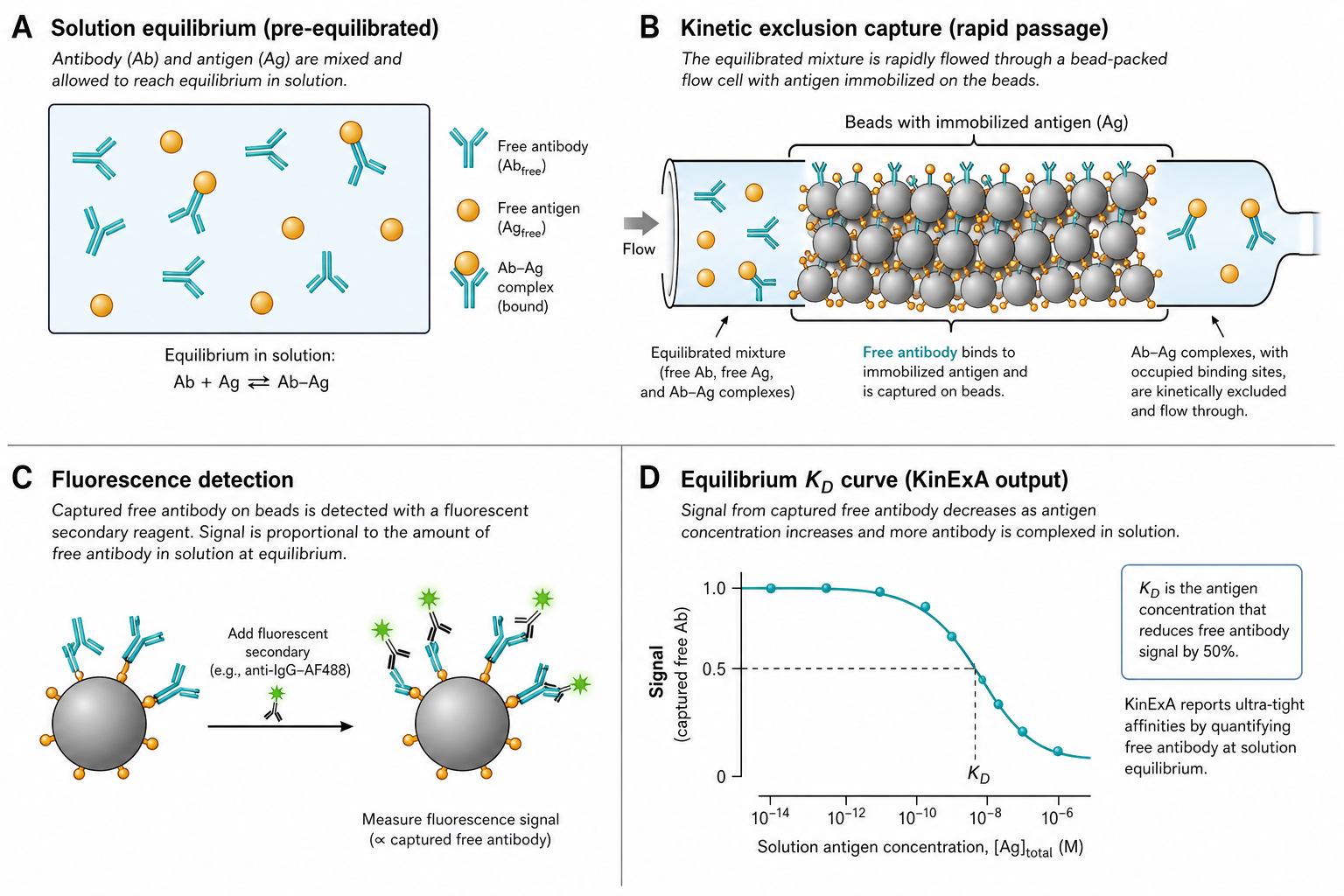
KinExA (Kinetic Exclusion Assay) measures the equilibrium dissociation constant KD of binding partners that stay unmodified in solution during the equilibrium itself. Antigen and antibody are mixed at known concentrations, allowed to reach equilibrium, and then briefly drawn through a column of antigen-coated beads. The contact time is too short for re-equilibration, so only the free antibody population is captured on the column and quantified by a labeled secondary. By titrating across many equilibrium mixtures, the free-antibody fraction is fit to the 1:1 binding quadratic to extract KD. The equilibrium pair never sees a label or a surface — though the assay itself still uses an antigen-coated bead column for capture and a labeled secondary for detection, both contacted only after equilibrium is reached.
Solution-phase equilibrium
The Ab–Ag equilibrium itself happens in free solution — no immobilization or tethering of either equilibrium partner. The bead column captures the free fraction post-equilibration; it does not perturb the equilibrium.
Unmodified equilibrium partners
The pair you characterize stays unlabeled and untethered through the binding event itself. (The assay still requires a coated bead column and a labeled detection reagent — they touch only after equilibrium is reached.)
Femtomolar KD
Sensitivity is set by how dilute you can run the receptor and still detect free signal — often pM, with fM achievable for high-quality systems.
Active concentration
Can determine the active fraction of binding sites independently of total protein — invaluable for batch QC.
Slow kinetics too
kon can be extracted from a kinetics curve (mixture sampled at multiple pre-equilibration times). Best for slow on-rates.
No equilibrium-step surface bias
The Ab–Ag equilibrium runs in solution, free of surface-mediated avidity and mass-transport bias. (Bead-capture artifacts — non-specific bead binding, free-Ab rebinding during transit at fast off-rates — still apply to the readout.)
Key Physics Concepts
⏱️ Kinetic Exclusion
- Pre-equilibrated mixture of antibody (Ab) and antigen (Ag) is drawn through an Ag-coated bead column
- Bead contact time (∼0.5–1.5 s) is much shorter than the complex's dissociation half-life
- Result: complexes survive intact through the column; only free Ab is captured
- Captured Ab is detected by a fluorescent secondary → signal ∝ free [Ab] in the equilibrium mixture
📉 KD- vs Receptor-Controlled Curves
- KD-controlled curve: [Ab] ≪ KD. Curve's midpoint is KD itself — direct readout of affinity
- Receptor-controlled curve: [Ab] ≫ KD. Curve's midpoint is set by [Ab] (stoichiometric titration) — gives active concentration of antigen
- Best practice: run several titrations at different [Ab] and fit them simultaneously — Sapidyne calls this an n-curve analysis. The combined fit constrains KD, [Ab]active, and [Ag]active at once
🐢 Slow Kinetics by Time Sampling
- Mix Ab + Ag and assay free Ab at multiple times before equilibrium is reached
- Free-Ab decay vs. time → fit a pseudo-first-order approach to equilibrium → extract kon (with KD from the equilibrium curve, koff = KD · kon)
- Particularly useful for slow on-rates (kon ≲ 10⁵ M⁻¹ s⁻¹) where SPR/BLI association windows are unhelpfully long
🧫 KinExA vs 📡 Surface Biosensors (SPR / BLI / GCI)
Solution equilibrium versus surface kinetics — different physics, different sweet spots.
| KinExA | SPR / BLI / GCI | |
|---|---|---|
| Format | Solution equilibrium + bead-column capture | Surface kinetics in real time |
| Modification | Equilibrium pair unmodified (capture beads + labeled detection still required) | One partner immobilized (often via tag/biotin) |
| Practical KD floor | Reaches fM with optimised, low-receptor titrations; pM is routine | Highly instrument- and analyte-dependent (≈pM at best with high-MW analytes, nM for fragments) |
| kon, koff | kon for slow systems; koff via KD · kon | Direct, real-time |
| Surface artifacts | No surface-mediated avidity or mass transport during the equilibrium step; bead-capture artifacts (NSB, residence-time bias for fast off-rates) still apply | Avidity, mass transport, rebinding for tight binders |
| Active concentration | Yes (k-curve) | Indirect (CFCA on some platforms) |
| Throughput | Low (hours per KD) | High (many samples in parallel) |
| Best for | Tight KD, unmodified pairs | Kinetics, screening, mid-range affinities |
How KinExA Works — Practical Guide
🔬 Experimental Setup
- Instrument: Sapidyne KinExA 4000 (current) or KinExA 3200 (earlier generation) — flow-based bead column with fluorescence detection
- Beads: Coat porous beads (e.g., azlactone or NHS-activated) with antigen at high density. Pack a small column for each measurement
- Equilibrium mixtures: series of vials at fixed [Ab] (well below expected KD for a KD-controlled curve), titrated [Ag]. Equilibrate (hours to days for tight systems)
- Sample volume: Larger volumes are pulled through the column to accumulate signal at low [Ab] — typically 0.5–10 mL per sample, scaling up to ~60 mL when chasing sub-pM KD (Bee et al. 2012)
- Detection: Labeled secondary antibody (anti-Ig, fluorophore) flows after the sample → signal ∝ free Ab captured
- Run: Each sample takes minutes; a full titration ranges from a few hours to overnight
📊 Data Analysis
- Free fraction: Normalize signal to the no-antigen control ([Ab]free / [Ab]T)
- Plot: Free fraction vs. log [Ag]T
- Fit: 1:1 quadratic binding equation → KD and active fractions
- Combine regimes: simultaneously fit a KD-controlled curve ([Ab] ≪ KD) and a receptor-controlled curve ([Ab] ≫ KD) — Sapidyne's "n-curve" analysis — for orthogonal constraints on KDand active concentrations
- Confidence interval: Sapidyne software returns 95% CI from bootstrap or profile-likelihood; report this, not just the point estimate
- Quality check: Inspect residuals; ensure curve spans the inflection in both directions
Key Quantities
| Quantity | Symbol | Typical range | What it tells you |
|---|---|---|---|
| Dissociation constant | KD | ~100 fM – 100 nM (sub-100 fM with heroic optimisation) | Equilibrium affinity |
| [Ab] for KD-controlled curve | [Ab]T | ≲ KD (often pM–fM for tight systems) | Sets sensitivity; lower [Ab] resolves smaller KD |
| [Ab] for receptor-controlled curve | [Ab]T | ≫ KD | Probes active [Ag] (stoichiometric titration) |
| Active fraction | factive | 0–1 | Fraction of protein that is binding-competent |
| Association rate | kon | 10³ – 10⁶ M⁻¹ s⁻¹ (the niche where SPR struggles) | From the time-course; KinExA's sweet spot is kon low enough that SPR association windows would be impractical |
| Dissociation rate | koff | ≲ 10⁻³ s⁻¹ | koff = KD · kon (derived) |
| Equilibration time | teq | Hours – days for tight systems | ~5/kobs; very tight pairs need long incubation |
| Sample volume | V | ~0.5–10 mL/run (up to ~60 mL for sub-pM binders) | Larger V at low [Ab] to build signal |
Common Pitfalls
Insufficient equilibration
For fM–pM KD, equilibration takes hours to days. Stopping early biases the apparent KD upward. Verify with a time-course at the lowest [Ag] used.
Fast dissociators
koff ≳ 10⁻² s⁻¹ starts to violate the kinetic-exclusion assumption — complexes dissociate during column transit and free-Ab fraction is biased high. KinExA is best for koff ≲ 10⁻³ s⁻¹; use SPR/BLI instead for faster off-rates.
[Ab] not low enough to resolve KD
If [Ab]T ≳ KD, the curve drifts into the receptor-controlled regime and KD is only bounded, not resolved. Drop [Ab] until the curve midpoint stops shifting with [Ab].
Bead saturation / non-specific binding
Over-coated beads or matrix binding cause baseline drift. Run buffer-only controls and validate with a non-binding isotype.
Active concentration error
Total [Ab] from absorbance ≠ active [Ab]. Run a receptor-controlled curve to determine active concentration and use it as a constraint when fitting the KD-controlled curve.
Bivalent antibody, monovalent KD?
IgGs are bivalent; reported KD is the monovalent intrinsic affinity only when antigen is monovalent and avidity is excluded. Check via Fab vs IgG comparison.
Adsorption to plasticware
fM–pM proteins lose to surfaces. Use low-bind tubes, carrier protein (BSA), and silanized glass where possible.
Reporting only the point estimate
Without a confidence interval, a fM KD claim is not interpretable. Always report 95% CI from bootstrap or profile-likelihood.
Strengths & Limitations
✅ Strengths
- • Femtomolar-to-picomolar KD, well below typical SPR/BLI floors
- • Equilibrium partners stay unmodified (capture beads + labeled detection only contact the sample after the equilibrium step)
- • No surface-mediated avidity or mass-transport bias during the equilibrium itself
- • Active concentration determination via the receptor-controlled (k-curve) regime
- • Combined fit of KD-controlled + receptor-controlled curves ("n-curve" simultaneous fit) constrains KD, active [Ab], and active [Ag] together
- • kon accessible for slow systems via time-course sampling
⚠️ Limitations
- • Low throughput — hours to overnight per KD
- • koff must be slow (t½ ≫ column transit time, typically koff ≲ 10⁻³ s⁻¹)
- • Not a real-time kinetics method — koff is derived, not observed
- • Single instrument vendor (Sapidyne)
- • Need a labeled secondary that recognizes the receptor (or direct label on Ab)
- • Sample consumption (mL volumes) higher than chip-based methods at high [Ab]
- • Bead-column preparation is part of the workflow — not plug-and-play
When to Use KinExA — and When Not
✅ Sub-pM affinities
Therapeutic antibodies, affinity-matured binders, anti-toxins. SPR/BLI floors leave you reporting only KD < limit.
✅ Tag-free equilibrium partners
When biotinylation or surface coupling of the binding pair perturbs binding (regulatory submissions, native-state characterization). The equilibrium partners stay untouched; the bead and detection reagents only contact the sample after the equilibrium step.
✅ Active-concentration QC
Lot release for biologics — KinExA k-curves give absolute active concentration.
⚠️ Fast off-rates
koff ≳ 10⁻² s⁻¹ starts to violate the kinetic-exclusion assumption (KinExA is best for koff ≲ 10⁻³ s⁻¹). Use SPR/BLI/GCI for faster off-rates.
⚠️ Need real-time kinetics
koff is derived (KD · kon), not observed. SPR is the right tool for kon, koff measurement.
⚠️ High-throughput screening
Hours per KD rules out primary screening campaigns. Use SPR/BLI/HTRF/ AlphaLISA upstream and confirm tight hits with KinExA.
Technique Comparison
| 🧫 KinExA | 📡 SPR | 🌊 FIDA | 🌡️ MST | |
|---|---|---|---|---|
| Format | In-solution + bead column | Surface-based (chip) | In-solution (capillary) | In-solution (capillary) |
| Modification | Equilibrium pair unmodified* | One partner immobilized | One partner labeled | One partner labeled |
| KD floor | fM, well-optimised | pM, MW-dependent | ~10–100 pM | pM–nM, MW/dye-dependent |
| Output | KD, active conc, kon (slow) | kon, koff, KD | Rh + KD | KD |
| Throughput | Low | High | Moderate | High |
| Best for | Tight KD, unmodified pairs | Kinetics | KD in crude matrices | Screening KD |
*KinExA: the equilibrium pair stays unmodified, but the assay still requires an antigen-coated bead column and a labeled detection reagent — both contacted only after equilibrium is reached.
Publication Checklist
🔬 Experimental
- ☐ Instrument and software version
- ☐ Bead chemistry and antigen coating density
- ☐ Antibody and antigen concentrations (each curve)
- ☐ Equilibration time and temperature
- ☐ Buffer / matrix composition
- ☐ Detection antibody and label
- ☐ Sample volume per measurement
- ☐ Number of replicates and curve types (n / k)
📊 Analysis
- ☐ Binding model (1:1) and fitting software
- ☐ KD with 95% CI (not just point estimate)
- ☐ Active concentrations from k-curve
- ☐ Combined n + k fit residuals
- ☐ Equilibration verified (time-course at lowest [Ag])
- ☐ Negative / non-binding controls
- ☐ kon (if reported) with method and time points
🔧 Instruments & Software
Instruments
- KinExA 4000 (Sapidyne Instruments) — current flagship. Auto-sampler, multi-position bead pack, fluorescence detection
- KinExA 3200 (Sapidyne Instruments) — earlier-generation instrument, still in widespread use
Software
- KinExA Pro (Sapidyne) — equilibrium & kinetics fitting, n/k-curve combination, confidence intervals
- Custom scripts — Python / R for non-1:1 models, global fits across constructs
Have SPR or BLI data?
Upload your raw files and get an automated kinetic analysis in minutes. We support Biacore, Octet, and other major formats.
Upload & Analyze