🟡 Localized Surface Plasmon Resonance (LSPR)
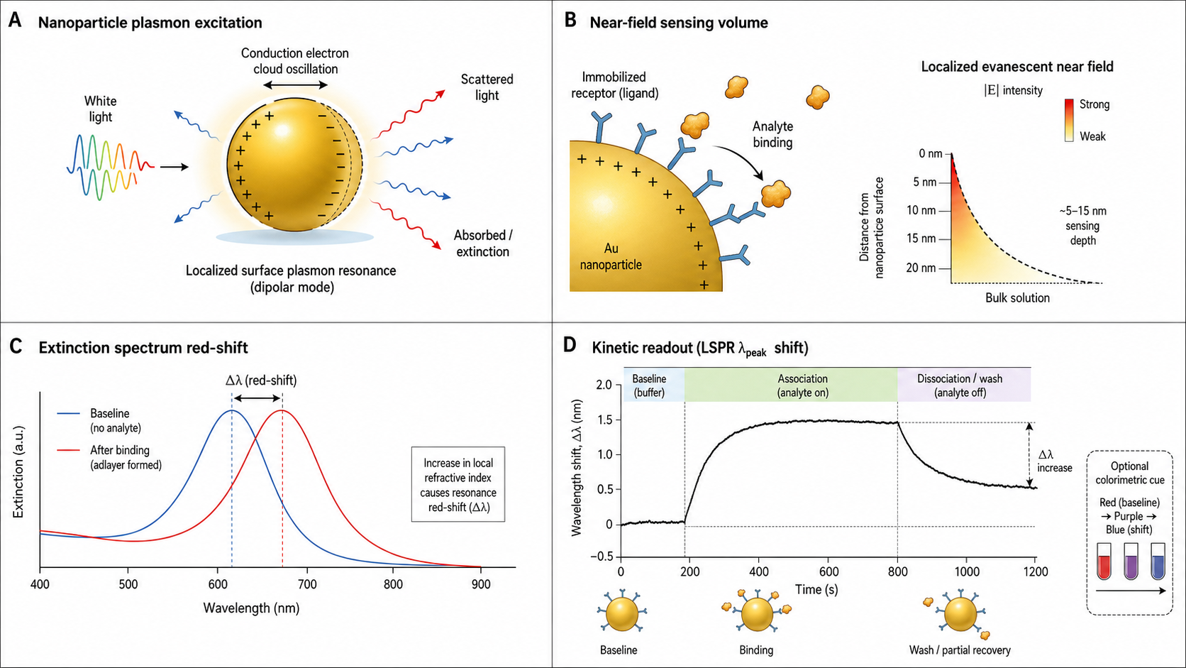
Shine white light through a solution of 40 nm gold nanoparticles and it turns wine-red. The particles are more than 10× smaller than the wavelength of visible light — yet they absorb and scatter specific colours with extraordinary efficiency. This is Localized Surface Plasmon Resonance (LSPR): the collective oscillation of conduction electrons in a metal nanoparticle driven by an incoming electromagnetic field, with a resonance frequency that depends exquisitely on particle size, shape, material, and chemical environment.
LSPR is the physics behind home pregnancy tests (the pink line is colloidal gold), rapid COVID diagnostics, and biosensors that detect single protein binding events in real time. Unlike propagating SPR, LSPR needs only a nanoparticle and a spectrometer. The short evanescent field (~5–15 nm vs SPR's ~200 nm) makes LSPR exquisitely sensitive to what's immediately on the particle surface and less dominated by distant bulk-solution changes than propagating SPR.
- Visible colour story: Resonance wavelength in the visible — you can literally see the sensor respond
- Extreme near-surface sensitivity: Evanescent decay ~5–15 nm: a protein monolayer fills the entire sensing volume
- No prism, no alignment: Simpler optical setup than SPR — a spectrometer and a cuvette is enough
- Tunable from UV to NIR: Change size, shape, or material to place the resonance anywhere in the spectrum
- SERS gateway: LSPR near-fields are the origin of surface-enhanced Raman scattering
Interactive Simulator
Adjust particle geometry and binding kinetics, then inject analyte to watch the nanoparticle colour shift and λ_max drift in real time.
Illustrative colour (display OD = 2)
Simulation speed: 10× real time | t = 0.0 s
Note: this simulator uses a quasi-static Mie/Gans approximation with Johnson & Christy 1972 optical constants. It includes an illustrative ensemble broadening term, but not full Mie retardation, radiation damping, or size-dependent scattering, so large-particle spectra remain qualitative.
Key Physics
The Fröhlich Condition
In the quasi-static limit (r ≪ λ), a metal nanoparticle is a polarizable sphere. Resonance occurs when the dipole polarizability denominator is minimised — the Fröhlich condition:
ε_r(ω) = −2 ε_m    where ε_m = n_m²

Au in water (ε_m ≈ 1.77):  ε_r ≈ −3.54 → resonance ~490–520 nm

Extinction cross-section:
  C_ext ∝ ε_i / [(ε_r + 2ε_m)² + ε_i²]
Replacing water (n = 1.333) with a protein layer (n ≈ 1.45) shifts ε_m upward, red-shifting the resonance. This is the LSPR sensing principle. Au's broad peak (~80–100 nm FWHM) reflects large ε_i from d-band interband transitions; Ag's peak is sharper because its interband threshold is in the UV.
Extinction is the sum of absorption and scattering: C_ext = C_abs + C_sca. The quasi-static expression above is the absorption cross-section in the small-particle limit. For r ≲ 25 nm extinction is almost entirely absorption (∝ V); for r ≳ 50 nm scattering (∝ V²) contributes substantially, broadening and red-shifting the peak via radiation damping. The strong scattering of larger nanoparticles is what makes single-particle dark-field LSPR sensing possible.
Dielectric data: uses Johnson & Christy (1972) tabulated n,k values, converted to ε(λ) = (n + ik)² on a 2 nm grid (380–1000 nm) — avoids Drude model double-counting of interband contributions.
⚠ For r < 10 nm: surface electron scattering broadens the linewidth (Kreibig correction: γ_eff = γ_bulk + A·v_F/r) — the simulator shows a warning badge but does not apply the correction.
Shape Effects — Tuning Across the Spectrum
Nanorods have two distinct plasmon modes:
- Transverse (~520 nm for Au, insensitive to aspect ratio)
- Longitudinal — red-shifts strongly with AR: λ_max ≈ 96 × AR + 418 nm (Link, Mohamed & El-Sayed 1999, Gans theory; coefficients shown are for ~10 nm-diameter Au rods in aqueous medium and shift with rod diameter and surrounding ε_m)
AR=2 → ~610 nm AR=3 → ~706 nm AR=4 → ~802 nm AR=5 → ~898 nm
The longitudinal mode also has higher bulk RI sensitivity (m ≈ 300–800 nm/RIU for rods vs ~100 nm/RIU for spheres). Nanoshells (silica core + gold shell) are tunable 600–1500 nm; nanostars have tip-localised hot spots giving SERS enhancement 10³–10⁴×.
| Shape | Material | λ_LSPR | Solution colour |
|---|---|---|---|
| 40 nm sphere | Au | ~520 nm | wine-red |
| 80 nm sphere | Au | ~548 nm | pink/purple |
| AR=3 rod | Au | ~706 nm | colourless (NIR) |
| 40 nm sphere | Ag | ~410 nm | yellow |
| Nanoprism | Au | 700–900 nm | blue/green |
LSPR Sensing — Wavelength Shift and Figure of Merit
Δλ_res = m × Δn × (1 − exp(−2d / l_d))

m    bulk RI sensitivity (nm/RIU)
     ~100       40 nm Au sphere
     ~300–600   Au nanorod (longitudinal)
Δn   n_layer − n_medium ≈ 0.117 (protein in water)
d    adlayer thickness (nm)
l_d  evanescent decay length ~ 0.2–0.5 × r (5–15 nm typical;
     shape- and geometry-dependent; Haes & Van Duyne 2004)

FOM = m / FWHM  (RIU⁻¹)
	     Au sphere  ~0.5–1.5    Au rod  ~3–8    Ag sphere  ~4–6
For a protein monolayer (d ≈ 5 nm) on 40 nm Au: Δλ ≈ 7 nm. Detectable limit ~0.3 nm → LOD ≈ few hundred pg/mm². Less sensitive than SPR per unit area, but the short l_d makes LSPR robust in complex biological matrices.
Applications
Point-of-Care Colorimetric Assays
Lateral-flow strips (pregnancy tests, COVID rapid tests) use antibody-conjugated 40 nm gold nanoparticles. Target-loaded particles are captured at an immobilized test line, concentrating a visible red line. 500M+ produced per year — no instruments, no power.
LSPR Biosensors
Nanoparticle arrays or colloid-functionalised chips with capture ligands. Track λ_max in real-time via transmission or dark-field spectroscopy. Commercial LSPR platforms include Insplorion XNano and LamdaGen LightPath. LSPR is especially useful when the assay benefits from short near-fields and simple optics. At the single-particle level, dark-field spectroscopy narrows the FWHM (~30–40 nm for Au) and raises the FOM 2–3× by removing ensemble polydispersity broadening. Note: Nicoya Alto (and their earlier OpenSPR) are conventional propagating-SPR instruments — not LSPR platforms despite the similar name.
SERS Substrates
Near-fields at nanoparticle junctions and nanostar tips amplify Raman scattering by 10⁶–10¹⁰. Designing SERS substrates requires understanding LSPR hot-spot geometry.
Photothermal Therapy
Gold nanorods absorb NIR light (800–1000 nm, tissue transparency window) and convert it to heat. Used in cancer therapy: particles accumulate in tumour, NIR laser irradiation causes selective thermal ablation.
Reading an LSPR Spectrum
| Observable | Meaning | Typical value |
|---|---|---|
| λ_max | Resonance wavelength — particle identity | 515–530 nm (Au sphere), 400–420 nm (Ag sphere) |
| FWHM | Linewidth — damping + polydispersity | 60–120 nm (Au), 30–60 nm (Ag) |
| Shoulder ≥ 650 nm | Aggregation, large particles, nanoprisms | Warning sign |
| Δλ on functionalization | Binding confirmed | 1–10 nm for monolayer |
| Dual peaks (rod) | Transverse (~520 nm) + longitudinal (variable) | Report binding from longitudinal peak |
LSPR vs Propagating SPR
| Feature | LSPR | Propagating SPR |
|---|---|---|
| Sensing element | Metal nanoparticle | Flat metal film |
| Optical coupling | Direct (no prism) | Prism (Kretschmann) |
| Evanescent depth l_d | ~5–15 nm | ~150–200 nm |
| Bulk RI sensitivity | ~100–800 nm/RIU | ~5,000–10,000 mdeg/RIU |
| Figure of merit | ~1–5 RIU⁻¹ | ~20–50 RIU⁻¹ |
| Best analyte size | Small proteins, peptides, small molecules | Any — proteins, complexes, cells |
| Complex matrix tolerance | High near-surface weighting | Moderate (referencing required) |
| Instrument cost | $5k–$100k | $100k–$500k |
Note: the LSPR sensitivity row is given in nm/RIU (wavelength-shift interrogation) while the SPR row is in mdeg/RIU (angle interrogation) — these aren't directly comparable. In wavelength-interrogated mode, SPR delivers ~3,000–9,000 nm/RIU. The figure-of-merit row normalises by linewidth and is the more meaningful side-by-side comparison.
Have SPR or BLI data?
Upload your raw files and get an automated kinetic analysis in minutes. We support Biacore, Octet, and other major formats.
Upload & Analyze