⚖️ Mass Photometry

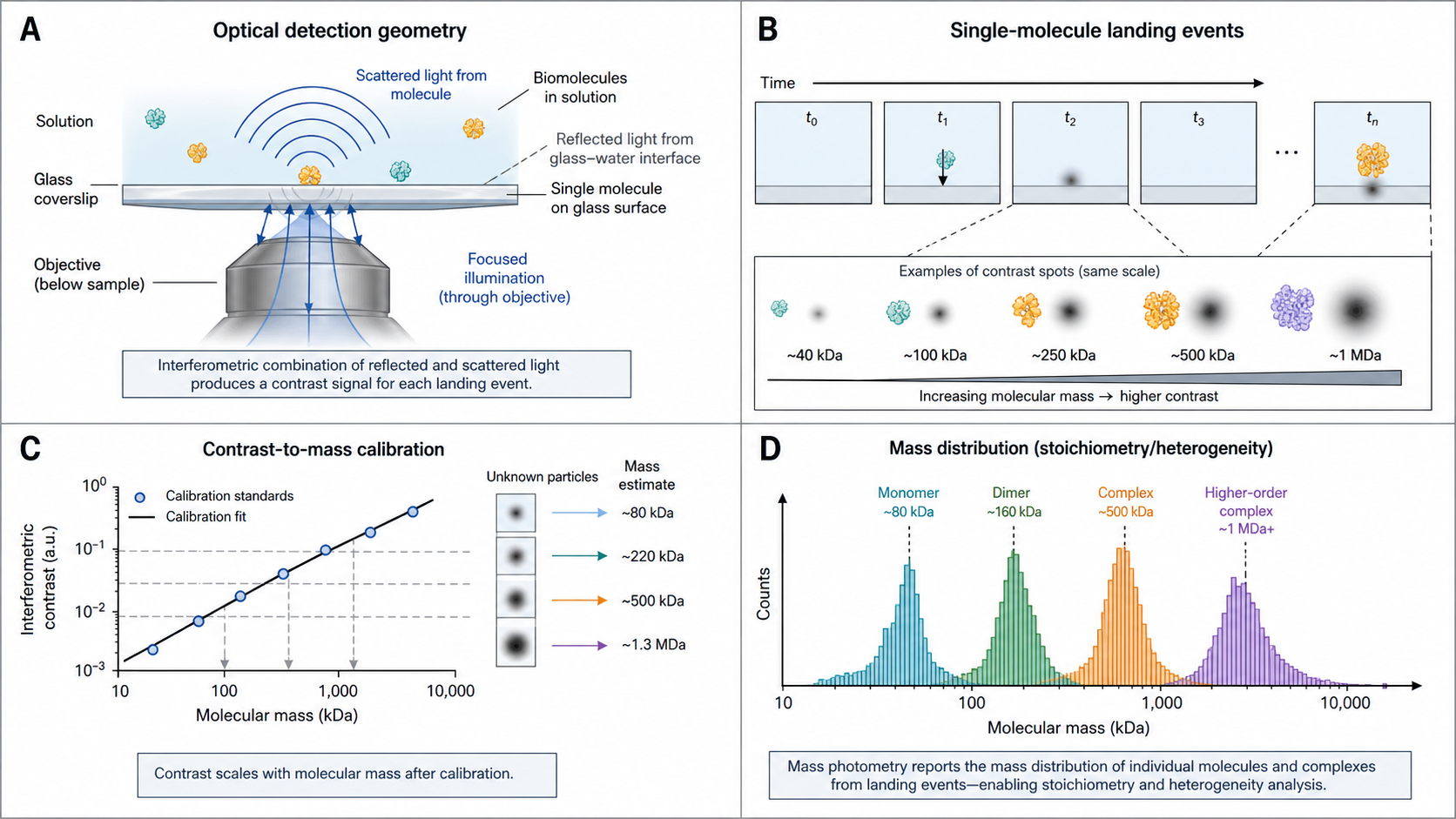
Mass Photometry (MP) measures the mass of individual biomolecules as they land on a glass surface. Each molecule that touches down scatters light, which interferes with the light reflected from the glass. The resulting interferometric contrast is directly proportional to the molecular mass — literally weighing single molecules with light.

Unlike ensemble methods (SEC, DLS, AUC) that report averages, MP sees every species individually. A 5% dimer contaminant that SEC might miss as a shoulder is a clear separate peak in MP. No labels, no columns, no immobilization — just drop 10–20 µL on a coverslip and record for 60 seconds.

Single-molecule sensitivity — see rare species (<5%)
60-second measurement — one histogram per minute
Native conditions — any aqueous buffer, no labels
Femtomoles to low picomoles of sample — 10–100 nM, 10–20 µL
Quantitative composition — peak areas ≈ molar ratios (see caveats below)

Key Physics Concepts

📏 Contrast-to-Mass Calibration

The raw signal is interferometric contrast (dimensionless, ~10⁻³–10⁻² for proteins).

Linear calibration: Contrast ∝ polarizability ∝ MW. Measure standards (66, 150, 669 kDa) → linear fit → MW = a × contrast + b.

Range: 30 kDa – 5 MDa routine spec; ≈20 kDa demonstrated in app notes / community usage on optimized samples, not the productized lower limit. Linear across the full range.

Accuracy: ±2–5% of expected mass. Competitive with native MS for large complexes where charge-state resolution becomes limiting; native MS retains superior mass accuracy (±0.01%) overall.

dn/dc: ~0.185 mL/g for proteins (standard). Heavily glycosylated proteins (dn/dc ~0.14–0.17) and detergent/lipid-bound complexes deviate depending on glycan or lipid content.

📊 Landing Events & Statistics

Each molecule landing on the coverslip = one data point. Build a mass histogram from hundreds of events.

Peak positions = species masses. Peak areas (counts) = molar fractions.

Landing rate: ∝ concentration × diffusion coefficient. Optimal: 200–800 events/min.

Statistics: Need ≥50–100 events per species for reliable peak assignment.

Counting: Every event is one molecule — peak areas give molar ratios directly, not mass ratios.

🔍 Mass Precision & Resolution

Can you distinguish two species?

Single-event σ: ~2–5% of MW for proteins >100 kDa. Instrument noise adds ~2 kDa baseline.

Resolution: Need ΔMW > 2σ to resolve two peaks. For IgG (σ ≈ 6.5 kDa): can resolve species ≥13 kDa apart.

Mean precision: σ_mean = σ_single/√N — improves with more events.

Resolution improves with mass — CV (σ/MW) decreases at higher MW.

σ ≈ 2 kDa + 3% × MW

Interactive Simulator

Differential image

Molecular weightkDa150 kDa

ConcentrationnM20 nM

Camera noiseLow

Frame averaging20 frames

Playback speed1×

Landing rate

0.6/s

SNR

10.1

Contrast

0.45%

Mass precision

±15 kDa

What you're seeing

Clear landing events — each dark speckle is a single protein hitting the glass. The darkening comes from destructive interference between scattered and reflected light. At 150 kDa, the contrast (0.45%) is well above the noise floor.

How Mass Photometry Works — Practical Guide

🧪 Sample Preparation

Coverslip: Clean borosilicate (#1.5H, 24×50 mm). Isopropanol + ddH₂O, dry with N₂. Or use CultureWell silicone gaskets (Grace Bio-Labs), as supplied by Refeyn.
Buffer: Any aqueous buffer. PBS, HEPES, Tris. Avoid: >0.01% detergent, >5% glycerol.
Focus: Add 10–20 µL buffer to coverslip. Find focus on the glass-water interface. Hardest part for new users.
Add protein: Add 1–2 µL concentrated stock into the buffer droplet → rapid dilution to 10–50 nM. Start recording immediately.
Record: 60 seconds standard. Collect 500–2000 events.

📊 Data Analysis

Event detection: Software identifies individual landing events (contrast spots appearing frame-to-frame).
Contrast extraction: Each event → one contrast value (peak of the PSF fit).
Calibration: Convert contrast → mass using calibration curve from known standards.
Histogram: Build mass histogram. Fit Gaussian peaks to identify species.
Quantification: Peak areas (counts) = molar ratios. Not mass ratios — each event is one molecule.
QC: Check >200 events, no high-mass tail, Gaussian peak shapes.

Concentration Optimization

The #1 mistake in mass photometry is wrong concentration.

Too dilute (<5 nM)

<50 events in 60 s → noisy histogram, poor statistics, unreliable peak fitting.

Optimal (10–50 nM)

200–800 events/min → clean histogram, reliable Gaussian fits, good statistics.

Too concentrated (>100 nM)

Simultaneous landings → artifactual peaks at 2× mass. If you see 2× peaks with pure sample, dilute.

Rule of thumb: Start at 20–50 nM. If landing rate >800/min → dilute 2×. If <100/min → concentrate 2×. Large complexes (>500 kDa): use 1–10 nM. MDa-scale assemblies scatter strongly enough to image down to ~100 pM. Small proteins (<50 kDa): may need 50–100 nM.

What MP Is Best At

✅ Heterogeneity analysis

See ALL species in solution, not just the average. A 5% dimer contaminant is a clear separate peak.

✅ Stoichiometry without labels

Mix A + B, see peaks at MW_A, MW_B, MW_AB. Direct read of complex formation.

✅ Quality control

Is your sample what you think it is? One measurement, 60 seconds, picomoles of protein.

✅ Complex assembly

Titrate subunits, watch the complex assemble. Sequential additions reveal assembly pathway.

✅ Equilibrium KD by titration

Vary analyte concentration and track bound-fraction populations to extract equilibrium KD — no immobilization required.

Key Quantities from MP

Quantity	Symbol	Typical range	What it tells you
Molecular mass	MW	30–5000+ kDa	Identity, oligomeric state
Mass precision	σ	2–5% of MW	Instrument & sample quality
Mass accuracy	ΔMW/MW	±2–5%	Calibration quality
Landing rate	events/min	200–800 optimal	Concentration adequacy
Species fraction	f_i	0–100%	Composition, purity
Mass resolution	ΔMW_min	~2σ ≈ 5–15 kDa	Ability to distinguish species

Common Pitfalls

1. Dirty coverslip

Non-specific binding → high background, false events. Always use fresh, cleaned coverslips.

2. Wrong concentration

Too high → double-landing artifacts at 2× mass. Too low → not enough events for statistics.

3. Buffer mismatch

Adding protein in different buffer → refractive index transient → artifacts in first 5 seconds.

4. Glycerol/detergent

>5% glycerol or >0.01% Tween → scattering background overwhelms signal.

5. Protein adsorption / surface charge

Sticky proteins deplete from solution → landing rate decays over time. Landing probability also depends on protein pI vs. coverslip surface charge, which can bias composition estimates for mixtures. Try PEGylated coverslips or adjust pH.

6. Not enough events

<200 events → can't reliably fit Gaussian peaks. Record longer or increase concentration.

7. Calibration drift

Calibrate same day, same coverslip batch. Laser power fluctuations shift contrast values.

8. Over-interpreting small peaks

Peaks with <30 events may be noise. Only report peaks with statistical significance.

Strengths & Limitations

✅ Strengths

Single-molecule sensitivity — see rare species (<5%)
60-second measurement
Native conditions — any aqueous buffer
No labels, no immobilization, no columns
Femtomoles of sample (10–20 µL at nM)
Direct stoichiometry from peak positions
Quantitative composition from event counts

❌ Limitations

Lower mass limit ~30 kDa routine (≈20 kDa reported in app notes on optimized samples, not the productized spec)
Mass accuracy ±2–5% (vs. ±0.01% for native MS)
Cannot distinguish isobaric species (same mass, different identity)
No shape/conformation information (unlike AUC)
Requires clean coverslips (consumable cost)
Narrow concentration window (~100 pM – 100 nM; 10–50 nM typical)
Kinetics limited to ~30-s time resolution by sequential snapshots (Soltermann 2020) — no real-time k_on/k_off like SPR/BLI
Lipid-nanodisc / membrane-protein complexes incur ~20% mass error without separate calibration (Olerinyova 2021)
Peak areas ≈ molar ratios only when landing probability is mass-independent; near the detection floor (~30–50 kDa) detection efficiency differences can introduce small bias
dn/dc deviations for nucleic acids, RNA, and membrane proteins in lipid nanodiscs — require separate calibration

When NOT to Use MP

❌ Small molecules (<30 kDa)

Below detection limit. Use native MS or MST instead.

❌ Exact mass (Da-level)

Need PTM identification or Da-level accuracy? Use native ESI-MS.

❌ Fast binding kinetics

MP supports ~30-s repeated-snapshot kinetics (Soltermann 2020) but not real-time k_on/k_off on sub-second scales. Use SPR or BLI.

❌ Concentrated formulations

Can't dilute to nM without shifting equilibria? Use DLS or SEC-MALS.

❌ Membrane proteins in micelles

Free detergent micelles scatter → noisy baseline. Use nanodiscs or SEC-MALS.

❌ Absolute quantification

MP counts molecules, not mg/mL. Use A280 or BCA for concentration.

MP vs Related Techniques

⚖️ Mass Photometry

• Single-molecule counting
• 30 kDa – 5 MDa
• ±2–5% accuracy
• 60 seconds
• 10–20 µL, 10–100 nM
• Any aqueous buffer
• Best for: quick heterogeneity

🔬 Native MS

• Population (ion ensemble, gas phase)
• 1 kDa – 10+ MDa (Orbitrap UHMR; 100+ MDa with CDMS)
• ±0.01% (Da-level)
• 5–30 min
• 5–10 µL, 1–10 µM
• Volatile buffers only
• Best for: exact mass, PTMs

📊 SEC-MALS

• Ensemble (solution)
• 1 kDa – 10 MDa
• ±5–10%
• 30–60 min
• 50–100 µL, 0.5–2 mg/mL
• Any SEC-compatible
• Best for: aggregation QC

⚙️ AUC

• Ensemble (solution)
• 1 kDa – 10 MDa
• ±5–10%
• 4–24 hours
• 400 µL, 0.1–1 mg/mL
• Any
• Best for: shape, sedimentation

Publication Checklist

Experimental Details

☐ Instrument stated (manufacturer, model)
☐ Coverslip preparation method stated
☐ Buffer composition stated
☐ Protein concentration at measurement stated
☐ Volume and mixing method stated
☐ Recording duration stated
☐ Calibration standards listed with masses
☐ Temperature stated (usually ~22°C)
☐ Number of replicates

Analysis & Results

☐ Software stated (with version)
☐ Calibration method and R² of fit
☐ Number of landing events per measurement
☐ Histogram shown with Gaussian fits
☐ Species masses and fractions ± SD reported
☐ Quality criteria stated (min events, max rate)
☐ Controls shown (buffer-only, individual components)
☐ Mass accuracy vs. expected noted

🔬 MP Instruments & Software

Instruments

Refeyn OneMP — Entry-level; 30 kDa lower limit; most widely used
Refeyn TwoMP — Enhanced sensitivity; 30 kDa routine spec (≈20 kDa achievable per app notes on optimized samples); temperature control; automated sample handling available

Software

Refeyn AcquireMP — Data acquisition
Refeyn DiscoverMP — Analysis, histogram fitting, calibration
Community scripts — Open-source Python analysis (see Refeyn GitHub and published supplement code)

Have SPR or BLI data?

Upload your raw files and get an automated kinetic analysis in minutes. We support Biacore, Octet, and other major formats.

Upload & Analyze