🧲 NMR Spectroscopy for Binding Studies
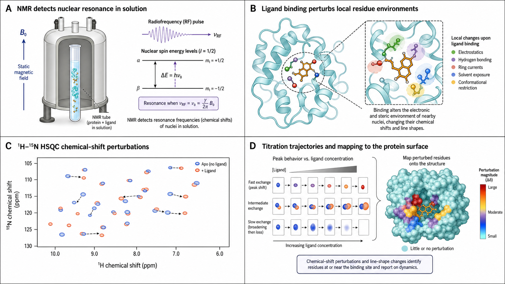
Nuclear Magnetic Resonance (NMR) spectroscopy provides atomic-resolution information on biomolecular interactions in solution, under near-physiological conditions. Unlike SPR/BLI (which measure mass changes at a surface) or ITC (which measures heat), NMR directly reports on local chemical environment changes at individual atoms upon binding. No immobilization. No surface artifacts. True solution-state measurement — you observe both binding partners in their native environment. NMR uniquely reveals where on the protein the ligand binds, which parts of the ligand contact the protein, and even the bound conformation of the ligand — structural detail accessible only through solution-state NMR.
NMR Exchange Regimes
A central concept for all NMR binding techniques is the exchange regime. It depends on the relationship between the exchange rate (kex = kon[L] + koff) and the chemical shift difference (Δω) between the free and bound states. The exchange regime dictates which NMR technique works best and what parameters are accessible.
| Regime | Condition | Typical KD (heuristic) | Spectral Appearance |
|---|---|---|---|
| Fast exchange | kex >> Δω | > ~100 µM | Single peak at population-weighted average position; peak shifts continuously during titration |
| Intermediate exchange | kex ≈ Δω | ~1–100 µM | Broadened or coalescing peaks — signals may disappear entirely at intermediate ratios |
| Slow exchange | kex << Δω | < ~1 µM | Two separate peaks (free and bound) whose intensities change with ligand concentration |
The exchange regime is set by the relationship between kex and Δω (in rad/s, or equivalently Δν in Hz), not by KD directly. The KD ranges above are rules of thumb that assume diffusion-limited kon (~10⁶–10⁸ M⁻¹s⁻¹) and ¹H/¹⁵N Δω of order 100–1000 Hz at typical fields (600–800 MHz); koff dominates kex once [L] is moderate. The regime is also nucleus-specific — the same binding event can appear as fast exchange for one residue and slow exchange for another, depending on the local Δω.
Key NMR Techniques for Binding
CSP (Chemical Shift Perturbation)
Record 15N-HSQC (Heteronuclear Single Quantum Coherence) spectra at increasing ligand concentrations. Peaks shift progressively in fast exchange. The magnitude and direction of shifts yield KD via titration fitting. 15N labeling required for 2D experiments; backbone assignment needed to map the binding site to specific residues but not for KD determination.
STD-NMR
Saturation Transfer Difference — selectively saturate protein resonances; saturation transfers to bound ligand via spin diffusion. The difference spectrum reveals which ligand protons contact the protein. No labeling required. Works at low protein concentration (1–50 µM) with large ligand excess (typically ~100×, to ensure unsaturated ligand replaces the departing one). For quantitative epitope mapping or KD estimation, use initial slopes of build-up curves rather than STDmax — a rapidly off-rating ligand can rebind while still partially saturated, inflating apparent STD at longer saturation times. For simple binding-vs-no-binding screening this is less critical. The gold standard for fragment screening in FBDD. STD and WaterLOGSY are prone to false positives from compound aggregation, non-specific binding, and detergent-like effects — counter-screen with apo (protein-free) controls and orthogonal competition experiments. See also rdSTD (reduced-dataset STD) for faster acquisition.
WaterLOGSY
Water-Ligand Observed via Gradient SpectroscopY — exploits magnetization transfer from bulk water through the protein–ligand complex. Binding ligands show opposite sign compared to non-binders. Complementary to STD with a different magnetization pathway. No labeling, low protein, qualitative binding readout.
CPMG Relaxation Dispersion
Carr-Purcell-Meiboom-Gill experiment measures how R2,eff varies with refocusing pulse frequency. Detects µs–ms exchange and extracts kex, populations, and |Δω| at a single static field. A second static field (or supplementary CEST/R1ρ data) is needed to remove sign/correlation ambiguity in Δω, since Rex scales with B₀². Together these methods provide kinetic rates and characterize invisible excited states.
trNOE (Transferred Nuclear Overhauser Effect)
Small ligands tumble fast (weak/positive NOE); when bound to a large protein, they experience slow tumbling (strong NOE with negative cross-relaxation rate, giving NOESY cross-peaks with same sign as diagonal). In fast exchange, bound-state NOEs dominate even at low bound fraction. Reveals the 3D conformation of the ligand in the binding pocket — unique to NMR.
PRE (Paramagnetic Relaxation Enhancement)
Attach a paramagnetic spin label to the protein. The unpaired electron causes distance-dependent relaxation enhancement (∝ 1/r6), useful out to ~20–25 Å for nitroxide spin labels (e.g. MTSL) and further still for lanthanide tags (Gd³⁺, Dy³⁺) — far exceeding the ~5 Å range of NOEs. Because of r⁻⁶ averaging weighted toward short distances, PRE is uniquely sensitive to sparsely populated states such as transient encounter complexes, and maps binding interfaces with long-range distance restraints.
Interactive NMR Simulator
Explore NMR binding experiments: chemical shift perturbation, exchange regimes, and STD build-up
CSP Titration Simulator
Simulate a ¹⁵N-HSQC titration experiment. Peaks shift along linear trajectories as ligand concentration increases (fast exchange regime). Color indicates [L]/[P] ratio.
The Combined Chemical Shift Perturbation
In a 1H-15N HSQC experiment, each residue gives a cross-peak at its unique (1H, 15N) coordinate. Upon ligand binding, peaks shift in both dimensions. The combined CSP collapses these two-dimensional shifts into a single metric:
Δδcombined = √( ΔδH² + (α · ΔδN)² )
Parameters
- ΔδH — change in 1H chemical shift (ppm)
- ΔδN — change in 15N chemical shift (ppm)
- α — normalizes the much larger 15N shift range against the smaller 1H range so both contribute meaningfully to the Euclidean distance. Values are derived either from gyromagnetic ratios (theoretical) or from BMRB shift-range statistics (empirical)
Common α Values
- ~0.10 — magnitude of |γN/γH| (γ ratio, theoretical); rarely used in practice because it under-weights 15N relative to its empirical shift dispersion
- 0.14 — Williamson (2013) recommendation based on BMRB statistical analysis of backbone amide shift distributions; most widely used for standard backbone CSP calculations
- 0.17 — Mulder et al. (1999) value derived from backbone amide pairs; seen in older literature
- 0.2 — commonly used empirical value (Farmer et al. 1996)
Residues with Δδcombined above a significance threshold (typically mean + 1–2 standard deviations) are mapped onto the protein structure to define the binding site.
KD from CSP Titration
In fast exchange only, the observed chemical shift perturbation is the population-weighted average: Δδobs = fbound × Δδmax (in slow exchange, peak intensities track binding — not positions — and this equation does not apply). For 1:1 binding (P + L ⇌ PL), the fraction bound follows the standard quadratic binding isotherm — the same equation used in ITC and fluorescence titration:
Δδobs = Δδmax × { ([P]₀ + [L]₀ + KD) − √( ([P]₀ + [L]₀ + KD)² − 4·[P]₀·[L]₀ ) } / (2·[P]₀)
Global Fitting
Fit multiple residues simultaneously sharing a single KD, with individual Δδmax per residue. This is analogous to global kinetic fitting of multiple SPR sensorgrams — the same principle of shared parameters with residue/concentration-specific observables. Consistency of KD across residues validates a single binding site.
Simplified Form
When [L]₀ >> [P]₀ (ligand in large excess), the equation simplifies to a hyperbolic saturation curve:
Δδobs = Δδmax × [L]₀ / (KD + [L]₀)
Reliable KD range: ~1 µM – 10 mM (fast exchange regime).
When to Use NMR vs SPR / BLI / ITC
🧲 Choose NMR when you need…
- Atomic-resolution binding site mapping — the only solution-state method providing true atomic-resolution mapping (requires 15N labeling; HDX-MS offers peptide-level resolution without labeling)
- Fragment screening — STD/WaterLOGSY are gold-standard for FBDD
- Weak binder detection — excels where SPR/BLI struggle (KD > 100 µM)
- Bound conformation — trNOE gives 3D structure of ligand in the binding pocket
- Aggregation/quality control — immediately reveals compound aggregation or protein unfolding
- Invisible excited states — CPMG detects transiently populated conformations invisible to other methods
✨ Choose SPR / 💡 BLI / 🌡️ ITC when you need…
- High-affinity KD — SPR/BLI measure down to pM; NMR limited to > ~1 µM
- Direct kinetics (kon, koff) — SPR/BLI provide real-time sensorgrams
- Thermodynamics (ΔH, ΔS) — ITC is the gold standard
- High throughput — SPR/BLI screen hundreds of analytes in hours
- Large proteins — no practical size limit for SPR/BLI/ITC
- Low sample consumption — SPR/BLI require µg quantities vs mg for NMR
Best practice: Use NMR and SPR/BLI/ITC together. NMR provides structural and binding site information; SPR/BLI provide precise kinetics; ITC provides thermodynamics. KD from multiple techniques should agree — orthogonal validation builds confidence in your results.
Practical Considerations
Sample Requirements
Protein-observed experiments (CSP, CPMG) require 0.1–0.5 mM protein (~200–500 µL), typically 15N-labeled. Ligand-observed experiments (STD, WaterLOGSY) need only 1–50 µM protein (unlabeled) with 20–100× ligand excess. Budget several mg of protein for a full CSP titration series. Buffer constraints: samples require 5–10% D₂O for field-frequency lock; use low-proton buffers (phosphate, Tris-d11, HEPES-d18) to minimize background. DMSO tolerance is typically ≤5% v/v for protein-observed experiments and up to ~10% for ligand-observed methods — exceed this and protein signal degrades markedly.
Molecular Weight Limits
Standard experiments work up to ~40 kDa. TROSY (Transverse Relaxation-Optimized SpectroscopY)-based experiments (requires 15N labeling; perdeuteration strongly recommended for proteins >30 kDa) extend the range to ~100 kDa or beyond. For systems above ~100 kDa (ribosomes, proteasome, GPCR complexes), methyl-TROSY with ILV/ILVA labelling (selective 13CH₃ labelling of Ile, Leu, Val, Ala methyl groups in an otherwise perdeuterated background) is the dominant approach, exploiting the favourable relaxation properties of methyl groups. Ligand-observed methods (STD, WaterLOGSY, trNOE) have no practical protein size limit — only the ligand needs to be NMR-visible.
Instrumentation & Cost
High-field NMR spectrometers (600–900 MHz) cost $1–5M. Cryoprobes increase sensitivity 3–4× (per scan; equivalent to ~10–16× time savings) but add cost. Single-field CPMG gives kex, populations, and |Δω|; a second field (or CEST/R1ρ) is needed only to resolve sign/correlation ambiguity in Δω. Most binding studies are performed at academic NMR facilities or pharma core labs. Expect $50–200/hour instrument time.
Common NMR Spectrometers for Binding Studies
Bruker Avance NEO — Most widely used platform for biomolecular NMR; available from 400 MHz up to 1.2 GHz (the latter with very limited installed base; 600–900 MHz most common) with cryoprobe options · Bruker Avance III HD — Predecessor to NEO, still widely installed in core facilities · JEOL ECZ Luminous — 400–950 MHz instruments with increasing adoption for biomolecular work · Bruker AVANCE Fragment Screening platform — Automated platform optimized for STD/WaterLOGSY-based compound screening
Have SPR or BLI data?
Upload your raw files and get an automated kinetic analysis in minutes. We support Biacore, Octet, and other major formats.
Upload & Analyze