〰️ SAW Biosensors
Surface Acoustic Wave (SAW) sensors confine acoustic energy to the surface of a piezoelectric substrate, rather than propagating through the bulk crystal as in QCM. This confinement dramatically increases mass sensitivity compared to bulk-wave devices. For biosensing in liquid environments, Love wave devices are the dominant SAW variant: a thin guiding layer (SiO₂ or polymer) on a piezoelectric substrate traps shear-horizontal waves at the surface, preventing radiation loss into the liquid.
Operating at frequencies of 80–300 MHz typical (with GHz devices in research) — well above QCM's 5–15 MHz — SAW devices achieve theoretical mass sensitivities that scale as f₀², making them attractive for detecting small molecules and low-abundance analytes. The planar lithographic fabrication enables mass production and potentially disposable sensor chips.
Higher mass sensitivity
Operating at 80–300 MHz, Love wave SAW achieves a practical LOD gain of ~10–100× over 5 MHz QCM.
Love wave confinement
Guiding layer traps acoustic energy at the surface — maximizing sensitivity while enabling liquid-phase operation.
Mass-producible
Planar lithographic fabrication (same as IC manufacturing) enables low-cost, disposable sensor chips.
Wet mass detection
Like QCM, SAW measures molecules plus coupled solvent — complementary information to optical (dry mass) methods.
Compact & portable
Small sensor footprint and simple electronics make SAW ideal for point-of-care and field-deployed diagnostics.
Key Physics Concepts
〰️ Surface Acoustic Waves
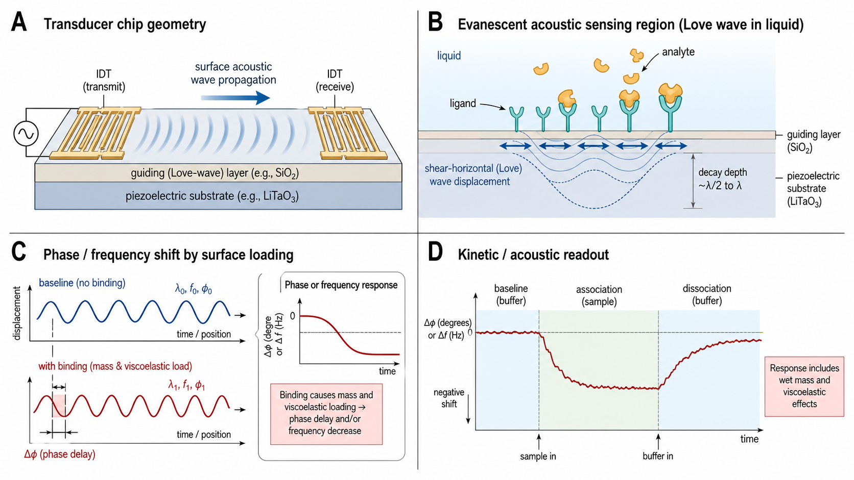
Interdigital transducers (IDTs) on a piezoelectric substrate (quartz, LiTaO₃, LiNbO₃) convert electrical signals into surface acoustic waves and back.
Rayleigh waves: Longitudinal + vertical shear components. Useful in gas phase but radiate energy into liquid, causing high damping.
SH-SAW: Shear-horizontal displacement — parallel to surface, no liquid compression. Enables liquid-phase operation.
Love waves: SH-SAW guided by a thin overlayer, concentrating energy at the sensing surface. The dominant mode for liquid-phase biosensing.
💎 Love Wave Sensors
A Love wave exists when a thin waveguide layer (SiO₂, PMMA, or SU-8, 1–5 μm thick) has a lower shear velocity than the substrate. This traps acoustic energy at the surface, dramatically enhancing mass sensitivity.
Sensitivity depends on layer thickness and frequency — there is an optimal thickness where sensitivity peaks. Named after mathematician A.E.H. Love (1911), who first described these guided waves in seismology.
⚖️ SAW vs QCM vs Optical
Higher frequency gives SAW higher mass sensitivity, but also higher noise — the sensitivity-to-noise ratio is what matters, not raw sensitivity alone.
SAW: Planar lithography, potentially disposable. Mass production. Limited viscoelastic characterization.
QCM-D: Simpler electronics, established Voigt modeling, more mature analysis software.
Optical (SPR, BLI): Measure dry mass via refractive index. Acoustic methods measure wet mass including coupled solvent.
IDT Design & Delay Line
An interdigital transducer consists of interlocking metallic "fingers" patterned on the piezoelectric substrate by photolithography. When an AC voltage is applied, the inverse piezoelectric effect generates a surface acoustic wave. The center frequency is determined by the electrode periodicity:
where v is the SAW velocity on the substrate (~4200–5100 m/s for SH-mode on common Love-wave cuts; Rayleigh modes on the same substrates sit lower) and λ is the acoustic wavelength set by the IDT geometry. The typical SAW biosensor uses a delay-line configuration: an input IDT generates the wave, which propagates across a sensing region where mass adsorption perturbs the wave, and an output IDT converts it back to an electrical signal.
Love Wave Structure
The Love wave biosensor is a layered structure optimized to confine acoustic energy at the sensing surface. The piezoelectric substrate provides the electromechanical coupling needed to launch and detect the wave. Common substrates include 36° YX-cut lithium tantalate (LiTaO₃) and ST-cut quartz.
The guiding layer is the key to Love wave operation. By depositing a material with lower shear wave velocity than the substrate, the acoustic energy becomes trapped near the surface — analogous to how a fiber-optic cladding confines light.
Above the guiding layer sits the functionalized sensing surface, where capture molecules are immobilized. When target analytes bind, the added mass shifts the wave's phase velocity and frequency — this shift is the measured biosensor signal.
Sensitivity & Detection
Like QCM, SAW mass sensitivity increases with operating frequency — for a rigid film, the frequency shift due to mass loading scales approximately as f₀². However, Love wave sensitivity is governed by acoustic perturbation theory, not the Sauerbrey equation (which applies to bulk-wave QCM), and depends critically on guiding layer optimization.
*Sauerbrey-extrapolated values assume f₀² scaling from bulk-wave QCM theory. Actual Love wave sensitivity depends on guiding layer optimization and is typically lower than these theoretical upper bounds.
Sensitivity vs. Noise
Raw sensitivity alone is misleading. Phase noise also increases with frequency, so the practical figure of merit is the limit of detection (LOD) — the minimum detectable mass change given the noise floor. Commercial Love wave LODs reference ~50 pg/cm² (0.05 ng/cm²), roughly 10–100× better than conventional 5 MHz QCM and approaching SPR.
Temperature Challenge
SAW frequencies drift substantially with temperature changes. Practical devices use a reference channel (a second delay line without receptors) for differential measurement, or employ temperature-compensated substrate cuts to minimize thermal drift.
Interactive SAW Explorer
Explore Love wave sensitivity, guiding layer optimization, and acoustic frequency scaling
Love Wave Sensitivity Explorer
Explore how operating frequency and guiding layer thickness affect Love wave mass sensitivity. The guiding layer creates an optimal thickness where sensitivity peaks — too thin and the wave isn't confined; too thick and higher-order modes appear.
Sensitivity vs. Guiding Layer Thickness
Applications
🧬 Biosensing
Love wave sensors have been demonstrated for detecting proteins, nucleic acids, and whole cells — primarily in buffer, diluted serum, or spiked samples. As pure mass sensors, SAW devices are inherently susceptible to nonspecific binding in complex matrices, requiring careful surface blocking and often sample dilution.
🏥 Point-of-Care Diagnostics
SAW's planar lithographic fabrication enables low-cost, mass-produced, potentially disposable sensor chips. Combined with compact electronics, this makes SAW attractive for portable diagnostic platforms — bringing lab-quality biosensing to the bedside or field.
💨 Gas Sensing & Industrial
In gas phase, Rayleigh-mode SAW devices excel at detecting volatile organic compounds, chemical warfare agents, and environmental pollutants. Wireless passive SAW sensors (no on-chip power needed) are used for industrial temperature and pressure monitoring in harsh environments.
Instruments using SAW
SAW Instruments GmbH (acquired by NanoTemper Technologies; sam®X platform status uncertain — no longer actively marketed) — formerly offered the sam®X Love wave biosensor with integrated microfluidics and multi-channel capability for label-free interaction analysis.
AWSensors — 120 MHz Love wave sensors compatible with their X1/X4 platform (same electronics as their HFF-QCM, different sensor chips). Dual-mode QCM + SAW capability.
Sandia National Labs / Academic — pioneered early SAW biosensor R&D. Many university groups fabricate custom SAW devices via lithographic prototyping; designs and protocols are widely published.
SenSanna — wireless passive SAW sensors for industrial monitoring (temperature, pressure, strain) in harsh environments. Demonstrates SAW versatility beyond biosensing.
Technology Comparison: SAW vs QCM-D vs SPR vs BLI
| Feature | SAW | QCM-D | SPR | BLI |
|---|---|---|---|---|
| Sensing Principle | Surface acoustic wave (mass) | Bulk shear wave (mass + viscoelasticity) | Surface plasmon resonance (refractive index) | White light interferometry (optical thickness) |
| Frequency Range | 80–300 MHz typical | 5 – 65 MHz (overtones) | N/A (optical) | N/A (optical) |
| Detection Limit | ~50 pg/cm² (commercial) | High (~0.5 ng/cm²) | Very high (sub-pg/mm²) | Good (pg/mm² range) |
| Viscoelastic Info | Limited (phase/amplitude) | Yes (ΔD + overtones → Voigt model) | No | No |
| Measures Coupled Water | Yes (acoustic) | Yes (acoustic) | No (optical) | No (optical) |
| Throughput | Low–Medium | Low (1–8 channels) | Low–Medium | High (96/384-well) |
| Sample Volume | μL (microfluidic) | μL (flow cell) | μL (flow cell) | μL (dip-and-read) |
| Commercial Maturity | Emerging | Established | Mature | Mature |
Acoustic vs Optical: What's the difference?
Optical methods (SPR, BLI) measure dry mass — refractive index changes proportional to the mass of adsorbed molecules alone. Acoustic methods (SAW, QCM-D) measure wet mass — the molecules plus hydrodynamically coupled solvent trapped in and around the adsorbed layer. For a protein monolayer, acoustic mass is typically 1.5–3× the optical mass; for DNA or polymer brushes, the ratio can reach 5–10×. Combining acoustic and optical measurements on the same surface enables direct quantification of hydration — a unique capability for understanding film structure.
Have SPR or BLI data?
Upload your raw files and get an automated kinetic analysis in minutes. We support Biacore, Octet, and other major formats.
Upload & Analyze