📸 SPR Imaging (SPRi)
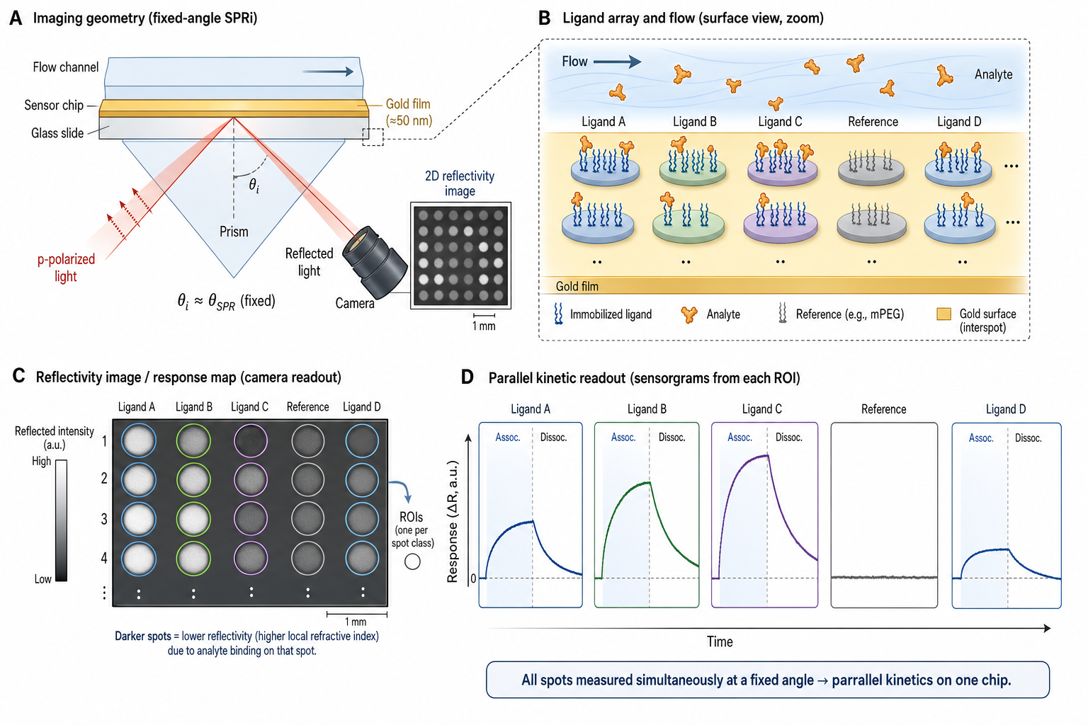
SPR Imaging (SPRi) extends conventional SPR from a single flow cell to a two-dimensional array of interaction spots, all monitored simultaneously by a CCD or CMOS camera. Instead of measuring reflected intensity at one spot with a photodiode, SPRi captures a full reflectivity image of the sensor surface — every pixel is an independent SPR measurement. This transforms SPR from a serial technique (one or a few interactions per run) into a massively parallel one (tens to hundreds of interactions per run).
The core physics is the same as classic SPR — p-polarized light in a Kretschmann (prism-coupling) geometry, evanescent field sensing refractive index changes at the gold surface — but the readout is fundamentally different. Instead of tracking the resonance angle of a single reflected beam, SPRi typically operates at a fixed angle near the SPR minimum and monitors reflectivity changes ΔR across the entire image. Each region of interest (ROI) drawn around a spot yields a sensorgram (ΔR vs. time), and the full set of sensorgrams forms a sensorgram map or kinetic heatmap.
Massive parallelism
100–400+ interactions per run. Entire antibody panels, mutant libraries, or epitope bins in one injection.
Built-in referencing
Interspot regions and dedicated reference spots on the same chip, under identical flow — best possible reference subtraction.
Spatial information
See heterogeneity across the surface. Bad spots, air bubbles, non-specific binding — all visible in the image.
Label-free kinetics
Same k_on, k_off, K_D as classic SPR, but for every spot simultaneously.
Efficient analyte use
One analyte injection interrogates all spots — 100× less sample than running 100 SPR cycles.
Key Physics Concepts
📐 Fixed-Angle Reflectivity
- Classic SPR tracks the resonance angle θSPR → high dynamic range
- SPRi operates at a fixed angle θ₀ near the SPR dip and monitors reflectivity R(θ₀)
- When molecules bind, θSPR shifts → reflectivity at θ₀ changes: ΔR ≈ (dR/dθ)|θ₀ × ΔθSPR
- Sensitivity ∝ slope dR/dθ at the working angle — maximum at the inflection point of R(θ)
- Operating wavelength: typically 660–850 nm (LED or laser); affects gold-thickness optimum, evanescent decay length, and per-RU sensitivity
- Evanescent decay length: ~150–300 nm at typical SPR wavelengths — bound mass at the surface dominates the signal; bulk RI further into the channel is largely rejected
- Conversion: 1 RU = 0.1 mdeg ≈ 1 pg/mm² (the mass conversion is the protein convention on CM-dextran at ~760 nm; nucleic acids and small molecules differ)
📷 Resolution vs. Sensitivity
- Spatial sampling: typically 2–10 µm/pixel pitch (optical resolution is coarser, ~10–30 µm). Spot diameters: 100–500 µm
- Larger ROI (more pixels averaged) → better SNR (∝ √Npixels) but coarser resolution
- Typical noise floor: ΔR ≈ 0.1–0.5% reflectivity per ROI; expressed in common units, this is roughly 5–50 RU equivalent (vs. < 0.1 RU for single-channel Biacore)
- Mass LOD: ~5–50 pg/mm² for SPRi vs. ~0.3–1 pg/mm² for Biacore (3σ) — i.e. ~10–100× less sensitive per spot
🎯 Array Referencing
- Killer advantage: every spot has neighbors that serve as references
- Double referencing: subtract (1) reference spot sensorgram and (2) buffer injection cycle
- Interspot referencing: bare gold between spots as local reference — accounts for bulk RI, drift, flow artifacts
- Spatial artifacts: non-uniform gold thickness, flow delay across array, depletion
Interactive Simulator
Left: Kretschmann prism coupling. Right: the camera's view. Move the angle — watch the reflection dim at resonance. Inject analyte — watch spots change as molecules bind.
R(θ) curve
How SPRi Works — Practical Guide
🔬 Array Preparation
- Gold chip: ~45–50 nm gold film on glass with a thin Cr (1–3 nm) or Ti (2–5 nm) adhesion layer. Standard SPR chips; some vendors supply pre-functionalized chips
- Surface chemistry: SAM of alkanethiols (e.g., 11-MUA), then activate with NHS/EDC. SPRi chips are often flat SAM (no dextran) for better imaging
- Spotting: Microarray spotter deposits ligands in a grid. Typical: 100–500 µm spots, 200–1000 µm pitch. Spotted in humid chamber, then quench
- Controls: Reference spots (blocked surface, irrelevant protein) in every row/column. Positive and negative controls. ≥3 replicates per ligand
- Mount: Assemble chip in flow cell. Prime with buffer. Equilibrate 10–30 min
📊 Data Acquisition & Analysis
- Set working angle: Scan angle to find θSPR, then offset to steepest part of the curve. Verify all ROIs show similar R₀ values
- Define ROIs: Draw regions around each spot and interspot reference. Software often auto-detects from contrast image
- Run cycle: Inject analyte → association → wash → dissociation. Repeat at 5–8 analyte concentrations
- Extract sensorgrams: Each ROI → ΔR(t). Apply double referencing
- Fit kinetics: Global fit to 1:1 Langmuir → kon, koff, KD per spot. Or steady-state if kinetics are too fast
- QC: Check mass transport, re-binding, spot heterogeneity, baseline drift
What SPRi Is Best At
✅ Antibody screening & ranking
Spot 100+ antibodies, inject antigen once → rank by K_D in a single experiment. Days of Biacore work in one run.
✅ Epitope binning
Sandwich/tandem assays across the full panel. N×N matrix of antibody pairs from N antibodies × N injections.
✅ Mutant library characterization
Spot all mutants, inject wild-type partner → see which mutations kill binding, which improve it.
✅ Array quality control
Image the surface — see missing spots, merged spots, uneven deposition before wasting analyte.
✅ Serum antibody profiling
Array of antigens, inject patient serum → map the full IgG/IgM reactivity profile in one experiment. Applicable to diagnostics, vaccine response, and autoimmunity research.
📐 Array Design Principles
Your SPRi experiment is only as good as your array layout.
- Replicate everything: ≥3 replicate spots per ligand, distributed across the chip (not clustered). Statistical rigor requires replication
- References in every row and column: Corner references alone can't correct for gradients across the chip
- Randomize positions: Avoid systematic position effects (upstream depletion, edge illumination)
- Control ligand density: Lower is usually better for kinetics (less mass transport). Target: 50–200 RU per spot
- Leave interspot gaps: ≥100 µm between spot edges for clean referencing
- Positive and negative controls: Include a known binder and a non-binding protein to bracket your expected range
Key Quantities
| Quantity | Symbol | Typical range | What it tells you |
|---|---|---|---|
| Reflectivity change | ΔR | 0.1–10% | Binding signal per spot |
| Resonance angle shift | ΔθSPR | 1–200 mdeg | Equivalent to classic SPR signal |
| Working angle offset | θ₀ − θSPR | 100–300 mdeg | Operating point on R(θ) curve |
| Sensitivity (slope) | dR/dθ | 0.1–0.5 %/mdeg | Conversion factor ΔR ↔ Δθ |
| Spot diameter | dspot | 100–500 µm | Determines pixels per ROI |
| Array size | Nspots | 16–400 | Throughput per run |
| Mass sensitivity | LOD | 5–50 pg/mm² | ~10–100× worse than single-channel SPR |
| KD | koff/kon | pM – µM | Same as classic SPR |
| Temporal resolution | Δt | 0.1–10 s | Frame rate; limits measurable kon at high [C] |
Common Pitfalls
Wrong working angle
Operating at the dip minimum (zero slope) → no sensitivity. Or too far away → poor sensitivity and nonlinear response. Always verify dR/dθ at each spot.
Non-uniform gold thickness
Even 1–2 nm variation shifts θ_SPR by ~0.1°. Spots at different positions may need different working angles. Use angle scanning to map θ_SPR across the chip.
Depletion across the array
High-density spots at the inlet consume analyte → downstream spots see lower [C]. Increase flow rate, lower ligand density, or account computationally.
Spot-to-spot variability
Non-uniform spotting (volume, contact time) → different ligand levels. Without replication you can't tell biology from spotting artifacts.
Insufficient referencing
Using only one reference spot for the whole chip fails if there are spatial gradients. Use interspot references distributed across the array.
Ignoring mass transport
SPRi spots often have higher ligand density than needed. If association looks linear (not curved), you're likely transport-limited. Lower ligand density.
Thermal drift
Chip temperature changes → θ_SPR drifts → baseline drift on ALL spots. Thermostat the instrument. Use fast referencing cycles.
Spot merging during printing
Humidity too high or volume too large → adjacent spots merge → cross-contaminated ligands. Optimize printing conditions on test chips first.
SPRi vs Related Techniques
📸 SPR Imaging
- • CCD/CMOS imaging of array
- • 100–400 spots/run
- • Label-free, real-time kinetics
- • LOD ~5–50 pg/mm²
- • k_on, k_off, K_D (all spots)
- • Fixed-angle mode → limited range; scanning-angle mode (e.g. IBIS MX96) → wide range
- • Best for: high-throughput screening
📡 Classic SPR (Biacore)
- • Photodiode, angle tracking
- • 1–16 ROIs/run (e.g. Biacore 8K: 8 channels × 2 spots)
- • Label-free, real-time kinetics
- • LOD ~0.3–1 pg/mm²
- • k_on, k_off, K_D (gold standard)
- • Angle tracking → wide range
- • Best for: detailed kinetics
🔬 BLI (Octet)
- • White-light interferometry
- • 8–96 sensors/run (parallel)
- • Label-free, real-time kinetics
- • LOD ~5–20 pg/mm²
- • k_on, k_off, K_D
- • Interference → wide range
- • Best for: crude samples, fast
🧊 Microarray (fluorescence)
- • Fluorescence scanner
- • 1000+ spots, endpoint
- • Labeled, endpoint (usually)
- • LOD ~1–10 pg/mL (solution)
- • K_D from titration only
- • N/A
- • Best for: discovery, serology
Strengths & Limitations
✅ Strengths
- • 100–400+ interactions per run — unmatched label-free throughput
- • Built-in spatial referencing — superior reference subtraction
- • See the surface — spot quality visible in real time
- • Efficient analyte use — one injection covers all spots
- • Same kinetic information (k_on, k_off, K_D) as classic SPR
- • Ideal for antibody panels, epitope binning, mutant screens
- • Spatial heterogeneity analysis within and between spots
⚠️ Limitations
- • ~10–100× less sensitive than single-channel SPR
- • Small molecule detection challenging (below noise floor)
- • Non-uniform gold → position-dependent sensitivity
- • Microarray printing adds complexity (spotting optimization, QC)
- • Limited dynamic range at fixed angle (~±2000 RU equivalent)
- • Array depletion artifacts in dense, high-density arrays
- • Fewer instrument vendors than Biacore
When NOT to Use SPRi
Detailed single-interaction kinetics
Need sub-0.1 RU noise? Use classic SPR (Biacore). SPRi sacrifices per-spot sensitivity for throughput.
Small molecule screening
Fragment hits (150–500 Da) produce ~1–5 RU on Biacore, below SPRi's noise floor. Use Biacore or signal enhancement.
Crude/unpurified analyte
Unlike BLI (dip-and-read), SPRi requires analyte to flow over the chip. Turbid samples scatter light and degrade image quality.
Very high affinity (K_D < 1 pM)
If k_off < 10⁻⁵ s⁻¹, dissociation is too slow (hours). Same limitation as classic SPR.
Quantitative concentration analysis
SPRi is calibrated in ΔR (arbitrary units per spot), not absolute concentration. Use ELISA or mass spec.
Membrane protein kinetics
Liposome or nanodisc-captured membrane proteins add optical complexity (scattering from lipid structures).
Publication Checklist
🔬 Experimental
- ☐ Instrument stated (manufacturer, model, camera specs)
- ☐ Gold chip type and functionalization chemistry
- ☐ Spotting method, spot diameter, pitch, volume per spot
- ☐ Array layout diagram (which ligand at which position)
- ☐ Number of replicates per ligand stated
- ☐ Reference spot strategy described
- ☐ Running buffer and analyte concentrations stated
- ☐ Working angle selection method stated
- ☐ Flow rate and temperature stated
📊 Analysis
- ☐ ROI selection method stated (manual/automatic, size)
- ☐ Referencing method stated (double referencing)
- ☐ Kinetic fitting model stated (1:1 Langmuir, etc.)
- ☐ k_on, k_off, K_D reported ± SD (across replicates)
- ☐ χ² or residuals for kinetic fits shown
- ☐ Sensorgrams shown (representative subset)
- ☐ Heatmap or array response summary shown
- ☐ Mass transport assessment described
- ☐ Spot quality criteria and excluded spots noted
- ☐ Comparison with single-channel SPR included if claiming quantitative KD agreement
🔧 SPRi Instruments & Software
Instruments
- Carterra LSA — High-throughput array SPR (HT-SPR). Produces up to a 384-ligand array via a 96-channel Continuous Flow Microspotter (CFM) printhead; ligands are spotted serially, not laid down on a fixed 384-spot chip. Gold standard for antibody screening
- IBIS MX96 — 96-spot SPRi. Angle scanning + fixed-angle modes. Commonly used with a CFM-style spotter (Wasatch Microfluidics / Carterra heritage) for array preparation
- Horiba OpenPlex — Compact SPRi with flexible array formats. Open surface access for custom spotting
- XelPleX (Horiba) — Multi-channel SPRi. Up to 4 independent fluidic channels on one chip
Software
- Carterra Kinetics — Automated ROI detection, kinetic fitting, epitope binning analysis
- IBIS Suite — Data acquisition and kinetic analysis for MX96
- Scrubber / TraceDrawer — Third-party SPR kinetic analysis tools compatible with SPRi data export
- Custom analysis — Python (scipy.optimize, matplotlib) or R
Have SPR or BLI data?
Upload your raw files and get an automated kinetic analysis in minutes. We support Biacore, Octet, and other major formats.
Upload & Analyze