💡 Bio-Layer Interferometry (BLI)

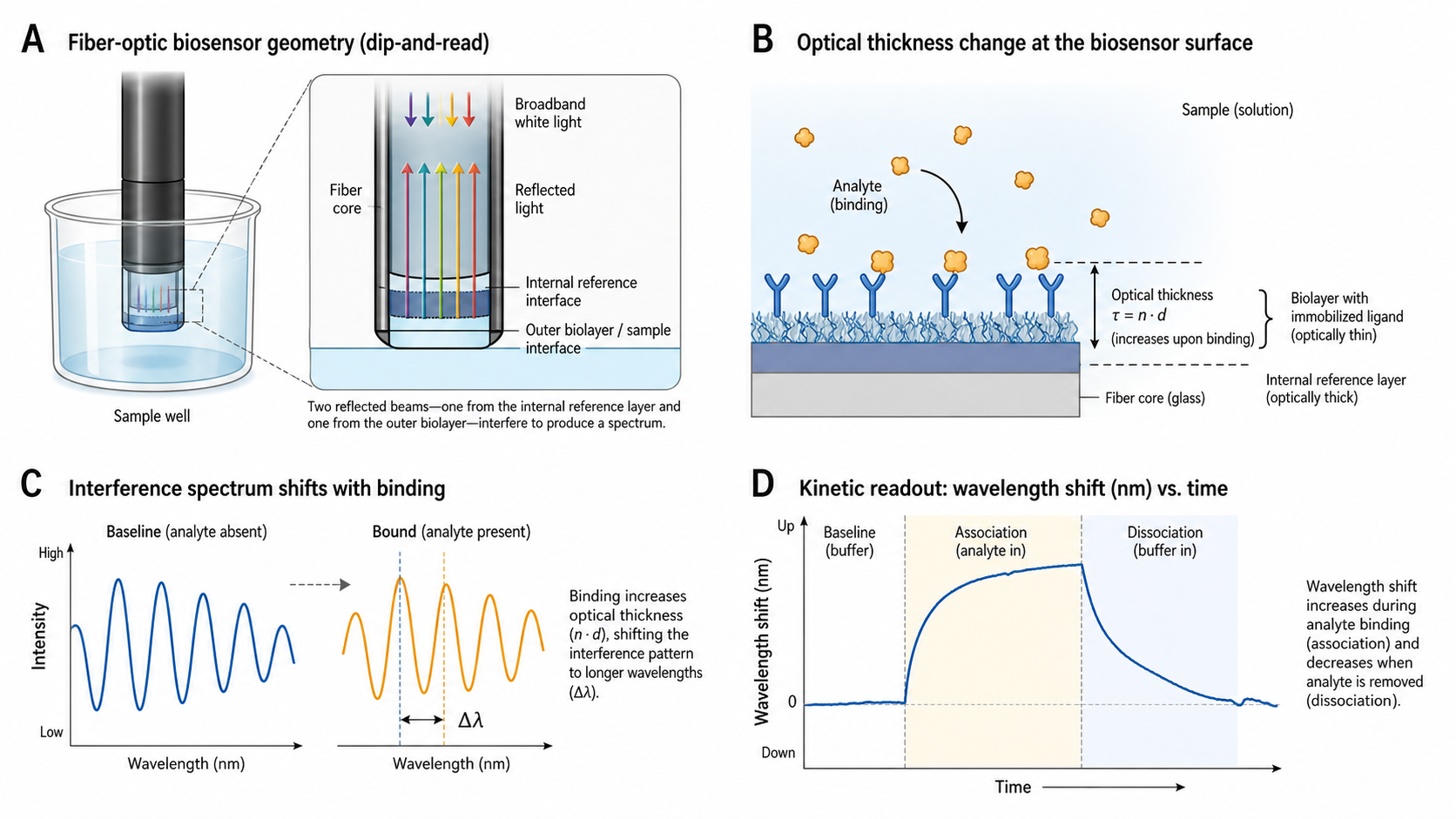
Figure 1 schematic explaining bio-layer interferometry: white-light reflection from a fiber-optic biosensor tip, interference between reference and bio-layer reflections, wavelength shift on binding, and kinetic sensorgram readout

Bio-Layer Interferometry (BLI) measures molecular binding by detecting changes in optical thickness at the tip of a fiber-optic biosensor. White light travels down the fiber and reflects from two surfaces: an internal reference layer and the outer bio-layer where molecules are immobilized. The interference pattern between these two reflections — a low-finesse two-surface thin-film interference geometry (only two reflecting surfaces, so the fringes are broad sinusoids, not the sharp peaks of a high-finesse cavity) — shifts in wavelength as molecules bind to or dissociate from the bio-layer surface.

Unlike SPR, BLI uses a dip-and-read format: sensors are physically dipped into microplate wells containing samples. This eliminates the need for microfluidics, makes BLI tolerant of crude and complex sample matrices (cell lysates, serum, hybridoma supernatants), and enables parallel measurements across 8, 16, or 96 sensors simultaneously — making it the dominant platform for high-throughput kinetics and affinity screening.

🔬

Optical thickness sensing

Measures the product of physical thickness × refractive index (n·d). Binding increases optical thickness, shifting the interference pattern.

⚡

Real-time kinetics

Monitor association and dissociation in real time. Extract ka, kd, and KD from multi-concentration kinetics experiments.

🧪

Dip-and-read format

No microfluidics — sensors dip directly into microplate wells. Tolerant of crude samples, particles, and viscous solutions.

🏭

High throughput

8–96 sensors run in parallel. Process hundreds of interactions per day with automated plate handling.

🏷️

Label-free detection

No fluorescent tags or reporters needed. Measure native molecules without modifying their structure or activity.

Key Physics Concepts

🌈 Thin-Film Interferometry

OPD = 2 · n · d

Light reflects from both surfaces of the bio-layer, creating an optical path difference (OPD) equal to twice the optical thickness (n × d). The resulting interference pattern — constructive at some wavelengths, destructive at others — is analyzed by a spectrometer.

When molecules bind, the bio-layer thickens and its average refractive index changes, increasing the OPD. This shifts the interference pattern to longer wavelengths — the measured "nm shift" is the BLI signal. Strictly, what is detected on binding is the change in index-contrast optical thickness, Δ[(n_layer − n_buffer) · d] — an index-matched layer (n_layer ≈ n_buffer) would produce no reflection at the layer/buffer interface and hence no signal, regardless of how thick it is.

🔬 Optical Thickness

Δλ ≈ 2 · Δ(n · d) / m

The BLI signal reports the change in optical thickness — the product of physical thickness and refractive index. Here m is the fringe order (the integer number of wavelengths in the optical path at the tracked feature). BLI cannot independently distinguish a thick, low-RI layer from a thin, high-RI layer.

For protein binding, a 1 nm BLI signal shift corresponds to roughly 1 ng/mm² of bound protein — analogous to ~1000 RU on SPR (Biacore), where 1 RU ≈ 1 pg/mm². Note that this is a shift on the BLI signal axis, not a 1 nm change in physical layer thickness: the actual layer growth that produces a 1 nm signal shift is much smaller, since optical thickness depends on the RI contrast between the layer (n ≈ 1.45) and water (n ≈ 1.33).

📊 Wavelength Shift

BLI instruments illuminate the sensor with broadband white light in the visible range (Octet systems span the visible, ~400–700 nm) and analyze the reflected spectrum. A spectrometer captures the full interference pattern and tracks the shift of specific fringe features over time.

The resulting sensorgram plots wavelength shift (nm) vs time — directly analogous to an SPR sensorgram (RU vs time). Association produces an increasing signal; dissociation produces a decreasing signal. Kinetic parameters are extracted by fitting to binding models.

Sensor Architecture

A BLI biosensor is a fiber-optic probe with a multi-layer optical coating at its tip. The coating creates the interference pattern; its outer surface is functionalized with capture molecules. Different sensor types use different surface chemistries for different immobilization strategies.

Optical fiber — delivers white light to the sensor tip and collects reflected light

Reference layer — internal, optically stable surface that provides one reflection

Bio-layer — outer surface where molecules are captured; its optical thickness changes upon binding

Signal — wavelength shift of the interference pattern, reported in nm

Interactive BLI Physics

Bio-Layer Interferometry Simulation

BLI Principle

White light reflects from two surfaces: a reference layer and the bio-layer surface. The two beams interfere, creating a wavelength-dependent pattern. When molecules bind, the bio-layer thickens, shifting the interference pattern — measured as a nm shift.

Sensor Layer Thickness1000 nm

600nm (fewer fringes)2000nm (more fringes)

Physical thickness of coating + streptavidin + ligand (n≈1.45)

Analyte Binding+0.0 nm

Sensitivity Scale

10× exaggerated for visibility

Sensor

1000 nm

+ Analyte

+0.0 nm

= Total

1000.0 nm

Measured Wavelength Shift

0.00 nm

Interference Spectrum (White Light Interferometry)

Pattern shifts right as binding increases optical thickness

Live Sensorgram

BLI vs SPR

• BLI: Measures optical thickness change directly (nm shift). No microfluidics needed — sensors dip into samples.
• SPR: Measures refractive index change in evanescent field. Higher sensitivity but requires flow system.
• Binding: Both detect mass changes at surface. 1 nm BLI shift ≈ ~1 ng/mm² ≈ ~1000 RU (SPR).
• Applications: BLI excels at crude samples, high-throughput screening. SPR better for detailed kinetics.
• Visualization: Bio-layer shown at exaggerated scale. Real optical thickness: 1000-1005nm.

Common Applications

🧬 Antibody Characterization

BLI's high throughput makes it the platform of choice for antibody screening campaigns. Epitope binning (competitive binding assays), affinity ranking of hundreds of clones, and detailed kinetics of lead candidates — all from crude hybridoma supernatants or cell lysates without purification.

💊 Drug Discovery

Hit validation and lead optimization. BLI is routinely used for quantitation assays (active concentration measurement), serum titer determination, and characterizing protein-protein interactions in drug target validation. The dip-and-read format enables testing in complex biological matrices.

🔬 Quantitation & QC

Rapid protein quantitation without calibration curves (using well-characterized capture sensors). Quality control of biologics: checking antigen-binding activity, lot-to-lot consistency, and stability under stress conditions. Fast turnaround: results in minutes, not hours.

Practical Considerations

Mass Transport & Shaking Speed

BLI relies on orbital shaking (typically 1000 rpm) to deliver analyte to the sensor tip. Unlike SPR's controlled laminar flow, BLI mass transport depends on shaking speed, well geometry, and sample volume. For accurate kinetics, use consistent shaking speeds and adequate sample volumes (≥200 μL in 96-well format). Very fast binders (k_a > 10⁶ M⁻¹s⁻¹) may be mass-transport limited.

Non-Specific Binding

Reference sensors (unloaded tips dipped in the same analyte) are essential for subtracting non-specific binding and bulk refractive index artifacts. Always include reference sensors in your assay layout. Double referencing (reference sensor + buffer-only analyte cycle) is recommended for high-quality kinetics data.

Loading Level Optimization

The amount of ligand loaded onto the sensor directly affects signal magnitude and kinetics quality. Overloading causes mass transport artifacts and rebinding during dissociation. For kinetics, target 0.5–1.5 nm of loading. For screening where signal-to-noise matters more, higher loading (2–4 nm) is acceptable.

Regeneration & Sensor Reuse

Some BLI sensors can be regenerated (analyte stripped, ligand retained) for multiple binding cycles. Common conditions: low pH (glycine-HCl pH 1.5), high salt, or specialized regeneration buffers. However, many BLI workflows use fresh sensors for each interaction — the disposable format is a key BLI advantage for crude samples.

Baseline Drift & Sensor Settling

BLI signals drift slowly over time due to sensor settling, temperature fluctuations, and evaporation from open microplate wells. For long dissociation phases (>30 min), evaporation in open wells can shift the baseline and distort k_d estimates. Allow sensors to equilibrate in assay buffer before baseline acquisition, use temperature-controlled plate holders where available, and keep dissociation times as short as the interaction permits.

Well-Transition Artefacts

Moving sensors between wells (dip-and-read) produces a characteristic refractive-index "jump" at each transition, as the sensor equilibrates to a new buffer or sample environment. These step artefacts must be excluded from kinetic fitting windows and are a primary reason double referencing is recommended — reference sensors undergo the same transitions and their signal can be subtracted.

Technology Comparison: BLI vs SPR vs GCI vs QCM-D

Feature	BLI	SPR	GCI	QCM-D
Sensing Principle	White light interferometry (optical thickness)	Surface plasmon resonance (RI)	Waveguide interferometry (RI)	Acoustic shear wave (mass + viscoelasticity)
Signal Unit	nm shift	RU (1 pg/mm²)	pm shift	Hz (Δf) + D (dissipation)
Detection Limit	~10 pg/mm²	~0.1 pg/mm²	~0.1 pg/mm²	~5 pg/mm² (0.5 ng/cm²)
Throughput	High (8–96 sensors parallel)	Low–Medium (1–8 channels)	Medium (up to 8 channels)	Low (1–8 channels)
Microfluidics	No (dip-and-read)	Yes (precise flow control)	Yes	Yes (flow cell)
Crude Sample Tolerance	Excellent	Limited (clogs fluidics)	Limited	Moderate
Kinetics Precision	Good (limited mass transport control)	Excellent (controlled flow)	Excellent	Moderate

Instruments using BLI

Sartorius Octet (formerly ForteBio) — current R-series: R2, R4, R8, R16, plus the high-throughput HTX (96-channel). Legacy platforms include the RED96, RED384, and QKe. The dominant BLI platform with an extensive sensor tip portfolio and Octet Analysis Studio software.

Gator Bio — GatorPrime (8-channel) and GatorPlus (16/32-channel). BLI instruments with competitive pricing and compatible sensor tips. Growing adoption in academic and biotech settings.

Key differentiator — All BLI instruments use disposable fiber-optic sensors, eliminating cross-contamination concerns and enabling direct measurement in crude matrices without pre-purification.