🔬 Microscale Thermophoresis (MST)

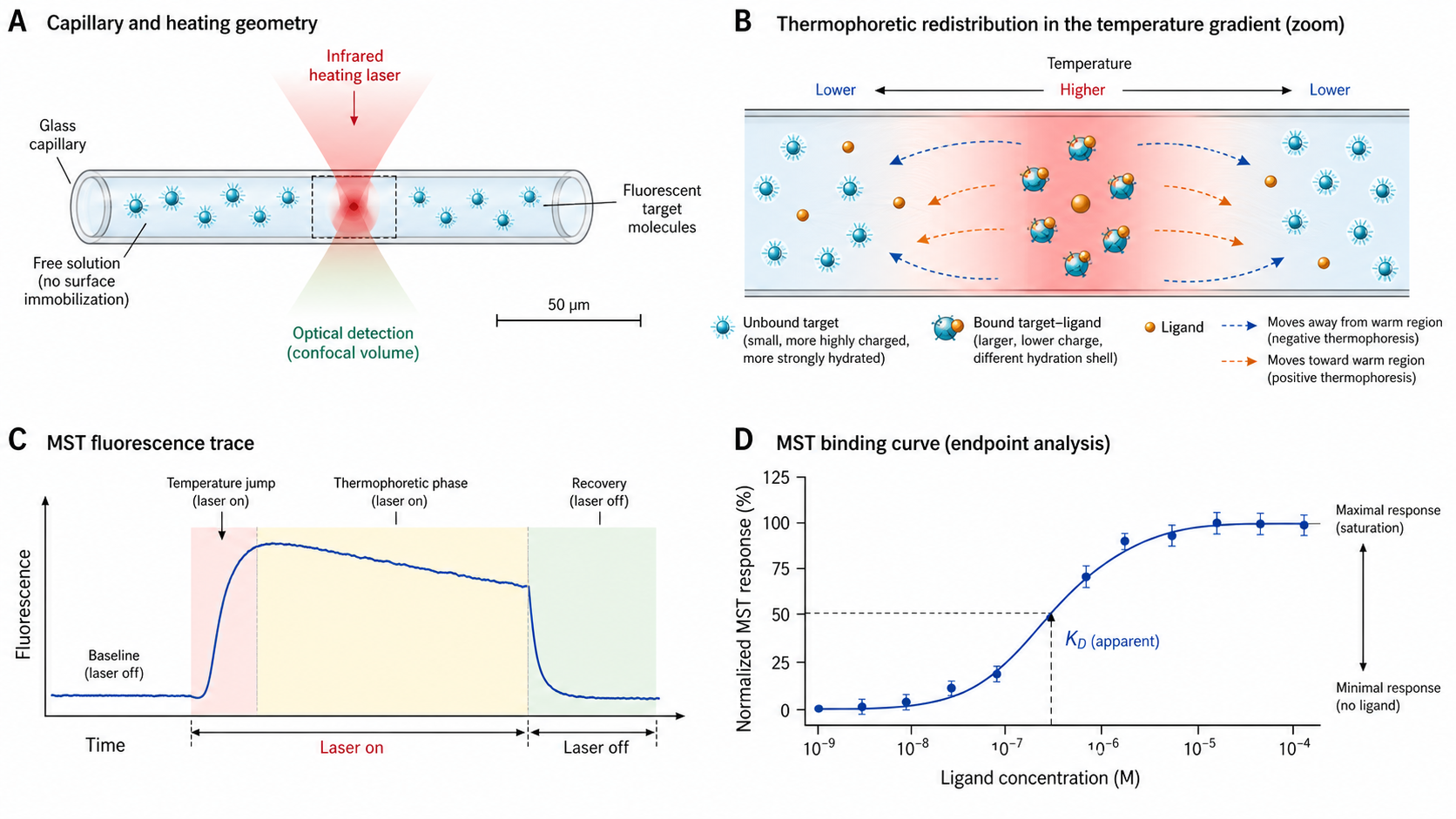
Figure 1 schematic explaining microscale thermophoresis: fluorescent target in capillaries, infrared laser temperature gradient, thermophoretic movement, fluorescence traces, and dose-response fitting

MST is one of the most versatile binding assays in biophysics: no surface, no size limit, works in crude lysates, and needs just microliters of sample. It measures molecular interactions in solution by detecting changes in the thermophoretic movement of fluorescently labeled molecules along a microscopic temperature gradient. When a ligand binds to the labeled target, it alters the target's size, charge, hydration shell, and conformation — all of which affect how the molecule moves in a temperature gradient. This change is detected as a shift in fluorescence distribution, yielding a dose-response curve from which the dissociation constant (K_D) is determined. No immobilization, no mass limitation — MST works in true solution with as little as ~4 µL of sample per capillary.

Key Physics Concepts

🌡️

Thermophoresis (Soret Effect)

Directed movement of molecules along a temperature gradient (Ludwig, 1856; Soret, 1879; modern MST foundations: Duhr & Braun, PNAS 2006; Wienken et al., Nat Commun 2010). Molecules typically move from hot to cold regions (positive Soret coefficient S_T), but S_T can also be negative under certain salt/temperature conditions (Iacopini & Piazza 2003), so the sign of ΔF_norm is not predictable a priori. S_T depends on molecular size, charge, hydration shell, and conformation — binding a ligand changes one or more of these, producing a measurable signal.

🔄

Binding-Induced Signal Change

When a ligand binds, the complex has different thermophoretic properties. Four contributors: size (complex is larger), charge (altered surface charge distribution), hydration shell (often the dominant factor — binding buries or exposes polar residues), and conformation (structural rearrangements). The weighted average of bound and unbound states produces a measurable shift in F_norm.

📈

Dose-Response Quantification

Titrate increasing concentrations of unlabeled ligand against a constant concentration of labeled target. Each concentration gives one F_norm value. Plot F_norm vs [Ligand] → sigmoidal dose-response curve → fit to binding isotherm → K_D. This is an equilibrium measurement — MST gives K_D but not kinetic rate constants (k_a, k_d).

🔬

Interactive MST Simulator

Explore microscale thermophoresis: fluorescence traces, dose-response curves, and experiment planning

Initial fluorescence — uniform distribution

Fluorescence Trace

Speed1.0×

Bound fraction40%

AnnotationsFluorescence trace

💡 Why do bound complexes move differently?

The Soret coefficient (S_T) determines how strongly a molecule is pushed by a temperature gradient. It depends on the molecule's size, charge, hydration shell, and conformation. When a ligand binds to the target, all four properties change — the complex is larger, its surface charge distribution shifts, and water molecules rearrange around it. In most cases, this increases S_T, causing the bound complex (orange) to deplete faster from the heated zone than the unbound target (cyan). However, the sign and magnitude of the change are empirical — some interactions decrease S_T or alter only the T-jump component. This differential behavior is what MST measures — the fluorescence change in the detection zone differs depending on how much target is bound.

MST Signal Phases

A single MST trace records fluorescence over ~40 seconds. Understanding the three distinct phases is essential for correct data analysis — and for distinguishing MST from related measurement modes (TRIC, Spectral Shift).

⚡ T-Jump (<1 s)

Rapid fluorescence change immediately after IR laser turns on. This is not thermophoresis — it reflects the temperature-related intensity change (TRIC) of the fluorophore: dominantly a quantum-yield shift, but modulated by the dye's local hydration shell and electronic environment, which is precisely why TRIC reports binding. Happens in <1 s. Some analyses use this phase alone (the "TRIC" evaluation).

🔬 Thermophoresis (5–30 s)

Gradual fluorescence change as molecules redistribute in the temperature gradient. This is the actual MST signal. Exponential approach to a steady state where thermophoretic drift and back-diffusion balance. Time constant τ_MST ≈ 5–15 s, depending on molecular size.

↩️ Back-Diffusion (5–20 s)

After the IR laser turns off, molecules diffuse back to a uniform distribution. Time constant τ_back ≈ 5–20 s (governed by Fick's law and molecular diffusion coefficient — larger molecules diffuse back more slowly). Not to be confused with thermal relaxation (~1–3 s).

🔑 MST vs TRIC vs Spectral Shift — Three Distinct Measurements

MST (Thermophoresis): Evaluates the slow thermophoretic phase (seconds). Measures how molecular properties change upon binding. The "classic" MST signal.

TRIC (T-jump): Evaluates only the fast temperature-dependent fluorescence change (<1 s). Detects binding through changes in the fluorophore's local environment. Often evaluated at 0.5–1.5 s after IR laser on.

Spectral Shift (Dianthus): Uses an extrinsic dye (e.g. RED-tris-NTA / RED-NHS) and measures the ratio of dye emission at two detection wavelengths (e.g. ~650/670 nm for the RED dye). No temperature gradient needed — detects binding-induced shifts in the dye's emission spectrum caused by changes in its local environment. Not thermophoresis, and not the same as nanoDSF's 330/350 nm intrinsic-tryptophan readout (Prometheus/Tycho).

How MST Works

The Measurement Principle

A focused IR laser (1480 nm, absorbed by water) creates a microscopic temperature gradient inside a glass capillary (~100–200 µm inner diameter). The heated spot is ~50–100 µm FWHM, producing a local temperature increase of 2–6 K. Labeled target molecules redistribute in this gradient (thermophoresis). Fluorescence is excited by an LED and measured by a detector — the ratio of fluorescence after thermophoresis to before gives F_norm.

From Traces to Binding Curve

Each capillary contains the same concentration of labeled target + a different concentration of unlabeled ligand. Typically 16 capillaries with 1:1 serial dilution. Each capillary produces one MST trace → one F_norm value. Plotting F_norm vs [Ligand] yields the dose-response curve, fitted to a 1:1 binding model (or Hill equation) to extract K_D. Signal-to-noise ratio (response amplitude / noise) determines measurement quality — SNR > 5 is the minimum threshold.

Labeling Strategies

MST requires a fluorescent signal. Choose your labeling approach based on your target protein and experimental goals. The decision tree below the cards helps you pick the right one.

🟢

Fluorescent Protein Fusions

GFP, EGFP, mCherry, YFP fused genetically to the target. Site-specific, homogeneous. Requires cloning and expression; tag may affect function.

Best for: Recombinant proteins already tagged. LED: Blue (470 nm) or green channel.

🔴

Chemical Labeling (NHS-ester)

NHS esters react with primary amines (lysine ε-amino groups). NanoTemper RED-NHS, Alexa Fluor 647, Cy5-NHS all work. Target degree of labeling (DOL) 0.5–1.0.

Best for: Any purified protein without His-tag. LED: Red (625–650 nm).

🏷️

His-tag Labeling (RED-tris-NTA)

Tris-NTA chelator binds 6×His-tag with low-nM affinity (typically ~1–10 nM, depending on tag length and Ni²⁺ loading). One-step, no purification needed. Works in crude lysates. Keep imidazole < 5–10 mM; no EDTA.

Best for: Rapid screening, crude lysates, His-tagged proteins.

🔶

Maleimide (Thiol-Reactive)

Reacts with cysteine sulfhydryl groups. More site-specific than NHS-ester labeling. Ideal when you have an accessible, non-essential cysteine or an engineered one.

Best for: Site-specific labeling when cysteine is available.

🧬

SNAP-tag / HaloTag

Self-labeling protein tags with fluorescent substrates. Very site-specific, highly efficient. Requires genetic fusion but offers excellent control over label position.

Best for: Precise site-specific labeling; growing in popularity.

⬜

Intrinsic Fluorescence (Label-Free)

Uses intrinsic tryptophan fluorescence (excitation ~280 nm). Truly label-free — no modification. Requires Trp residues near the binding site. Lower sensitivity, higher protein concentrations needed (100 nM–10 µM). Requires UV optics (NT.LabelFree).

Best for: Membrane proteins, native protein validation.

🌳 Choosing Your Labeling Strategy

Is your protein His-tagged?

→ YES: RED-tris-NTA (fastest, works in lysate)

→ NO: Is it already a fluorescent fusion (GFP, mCherry)?

→ YES: Use the FP channel

→ NO: Is purified protein available?

→ YES, accessible Cys: Maleimide dye

→ YES, no specific Cys: NHS-ester dye (RED-NHS)

→ NO: Can you add a tag? → SNAP/HaloTag or His-tag

→ NO modification possible: Intrinsic Trp fluorescence (UV)

Experimental Design — Step-by-Step Protocol

10-Step MST Protocol

Choose labeling strategy — use the decision tree above
Label your target — follow the protocol for your chosen approach; verify activity post-labeling
Determine optimal [Target] — run an LED scan; aim for 200–2000 fluorescence counts; use ≤ K_D/10 if possible
Prepare serial dilution — 16 points, 1:1 dilution; range from ~20× above to ~20× below expected K_D
Mix target + ligand — combine equal volumes; allow equilibration (10–15 min at RT)
Load capillaries — standard treated (default), premium coated (sticky proteins), or hydrophobic (membrane proteins)
Run capillary scan — check for aggregation (spikes) and adsorption (decreasing fluorescence)
Run MST measurement — set LED power, MST power (start at Medium), evaluation time
Fit dose-response — calculate F_norm, fit to 1:1 model (quadratic if [Target] > K_D/10)
Validate — run SD-test, negative control, ≥ 3 independent replicates

Buffer & Capillary Optimization

Recommended starting buffer: 50 mM HEPES pH 7.4, 150 mM NaCl, 0.05% Tween-20. Match buffer between target and ligand samples exactly.

Tween-20/Pluronic F-127 (0.01–0.05%) — prevents adsorption
BSA (0.05–0.5 mg/mL) — anti-adsorption, if not interfering
DMSO — tolerated up to ~5%; keep constant across all points
Salt — high salt (>500 mM) can reduce electrostatic MST signal
Imidazole — keep <5–10 mM for His-tag labeling

Capillary Types

Standard Treated — hydrophilic, general purpose (default)
Premium Coated — enhanced hydrophilic, for sticky/low-conc proteins
Hydrophobic — for membrane proteins in detergent

⚡ MST Power Settings

MST Power = IR laser intensity. Higher power → stronger signal but more risk of artifacts.

Low (20%) — Minimal heating. Use for thermally sensitive proteins or when artifacts appear at higher power.

Medium (40%) — Default starting point. Good balance of signal and minimal artifacts.

High (80%) — Maximum signal. Use when signal is weak. Risk of aggregation, unfolding, convection.

The Concentration Rule — MST's Design Parameter

Just as ITC has the Wiseman c-value, MST has a critical design parameter: the ratio of target concentration to K_D. Getting this wrong is the #1 source of incorrect K_D values.

[Target] ≤ K_D/10 — Ideal

Ligand depletion is negligible. Simple binding model works. EC₅₀ ≈ K_D. This is the sweet spot.

[Target] = K_D/10 to K_D — Use Quadratic

Some ligand depletion. EC₅₀ shifts right. Use the quadratic binding model and report this. K_D is still reliable.

[Target] >> K_D — Danger Zone

Severe ligand depletion. Apparent K_D ≈ [Target]/2 regardless of actual affinity. You're measuring stoichiometry, not affinity. Reduce [Target] or report K_D as an upper limit.

Data Analysis

F_norm — The MST Observable

F_norm = F_hot / F_initial × 1000 [‰]

F_initial = average fluorescence before IR laser ON (baseline). F_hot = average fluorescence at a defined time after IR laser ON. Two common evaluation windows:

T-jump evaluation (~0.5–1.5 s): Captures temperature-dependent fluorescence change only (TRIC)
MST + T-jump (~1.5–5 s): Captures thermophoretic movement + T-jump

ΔF_norm = F_norm(bound) − F_norm(unbound). Typical response amplitudes: 5–100‰. A ΔF_norm of 10‰ is a decent signal.

Note: F_norm in ‰ is NanoTemper's convention. Other groups may report ΔF/F or alternative normalizations.

1:1 Binding Models

Simple (no ligand depletion): When [Target] ≪ K_D:

f_bound = [L] / ([L] + K_D)

Quadratic (with ligand depletion): When [Target] is significant relative to K_D:

f_bound = {([L]+[T]+K_D) − √(([L]+[T]+K_D)²−4[L][T])} / (2[T])

The signal equation: F_norm([L]) = (1−f) · F_norm,unbound + f · F_norm,bound

Hill & Competition Models

Hill equation (cooperative binding):

f_bound = [L]ⁿ / ([L]ⁿ + K_D,appⁿ)

n > 1: positive cooperativity. n < 1: negative cooperativity or heterogeneous population. K_D,app is not a true microscopic K_D.

Competition assays — Cheng-Prusoff equation:

K_i = IC₅₀ / (1 + [A] / K_D,A)

Caveat: assumes competitive (same-site) binding and that [A] ≈ free [A]. Does not apply to non-competitive/allosteric displacement.

Quality Assessment Criteria

Metric	Good	Acceptable	Poor
Signal-to-noise (ΔF_norm/σ)	>12	5–12	<5
Response amplitude (ΔF_norm)	>20‰	10–20‰	<10‰
Capillary scan shape	Flat, uniform	Minor variation	Spikes, irregular
Fluorescence consistency	<10% variation	10–20%	>20%
K_D confidence (68% CI)	<3-fold	3–10-fold	>10-fold

Data Interpretation — Good vs Bad MST Data

Learning to read MST data takes practice. Here are three realistic scenarios showing what to look for and how to troubleshoot.

✅ Good Data

Traces: Smooth, reproducible across replicates. Clear T-jump + steady thermophoretic plateau. No bumps or irregularities.
Capillary scan: Flat, uniform fluorescence. No spikes. <10% variation between capillaries.
Dose-response: Clean sigmoidal curve. Both plateaus well-defined (unbound baseline and saturated response). ΔF_norm > 20‰, SNR > 12.
K_D: 150 ± 30 nM (68% CI within 3-fold). [Target] = 10 nM — well below K_D/10. Simple model is valid.

→ Publish-ready.

⚠️ Fixable Problems

Symptom: Initial fluorescence drops by 30% across capillaries (high [ligand] → low [ligand]). Traces look OK otherwise.
Diagnosis: Protein adsorption at low ligand concentrations — the ligand may stabilize the protein against surface sticking.
Fix 1: Add 0.05% Tween-20 to the buffer.
Fix 2: Switch to premium coated capillaries.
Fix 3: If fluorescence variation persists, add 0.5 mg/mL BSA.

→ Re-measure after buffer fix.

❌ Misleading Data

Symptom: Beautiful sigmoidal curve, K_D = 250 nM. But [Target] = 500 nM → K_D ≈ [Target]/2.
Diagnosis: Severe ligand depletion. You're measuring stoichiometry, not affinity. The real K_D could be 10× lower.
Red flag: K_D always tracks [Target] — halve the protein, K_D halves too.
Fix: Reduce [Target] to ≤ K_D,estimated/10. If fluorescence is too low, use the quadratic model and report the [Target] used.

→ Do NOT publish. Re-optimize.

Quality Control & Troubleshooting

🔴 Ligand-Induced Fluorescence

Symptom: Initial fluorescence varies systematically with [ligand]. Cause: Ligand quenches/enhances the dye or is itself fluorescent. Fix: Different labeling position; check ligand spectrum; run SD-test.

🔴 Buffer Mismatch

Symptom: Systematic F_norm drift correlated with ligand dilution (not sigmoidal). Cause: Ligand in different buffer (DMSO/glycerol gradient). Fix: Ensure identical buffer in all points; run buffer-only control.

🟡 Adsorption to Capillary Walls

Symptom: Decreasing initial fluorescence at low [ligand]. Cause: Protein sticks to glass. Fix: Add 0.01–0.05% Tween-20; add BSA; use premium coated capillaries.

🟡 Aggregation

Symptom: Irregular traces, fluorescence spikes in capillary scan. Cause: Protein aggregation from heating or high concentration. Fix: Centrifuge samples; reduce MST power; more detergent.

🟡 Photobleaching

Symptom: Fluorescence decreases over time within a trace; baseline drifts down. Cause: Fluorophore degradation from excitation light. Fix: Reduce LED power; use photostable dyes (Cy5 > fluorescein).

🟡 Capillary Scan Irregularities

Symptom: Non-uniform fluorescence distribution (peaks, shoulders). Cause: Protein adsorption creating fluorescent hot spots. Fix: More detergent; premium coated capillaries; different type.

🟡 Protein Unfolding

Symptom: Irreversible fluorescence changes after IR exposure. Cause: 2–6 K increase may unfold marginally stable proteins. Fix: Lower MST power; verify stability with nanoDSF/Tycho at T_m + 6K.

🟡 Convection

Symptom: Irregular, non-reproducible trace shapes between identical samples. Cause: Convective flow in unsealed or over-heated capillaries. Fix: Ensure proper sealing; reduce MST power.

✅ The SD-Test (SDS Denaturation)

Add SDS (1–4% w/v) + DTT to the labeled protein. SDS denatures the protein → destroys the binding site. If the MST signal disappears, the signal was likely binding-specific. If it persists, it may be a dye artifact. This is a necessary but not sufficient control — run it for every new interaction.

When NOT to Use MST

MST is versatile, but it's not the right tool for every experiment. Honest assessment:

❌ When you need kinetics. MST gives only K_D — no k_a, k_d, or residence time. Use SPR or BLI for kinetic characterization.

❌ When you need thermodynamics. MST gives no ΔH, ΔS, or direct stoichiometry. Use ITC for complete thermodynamic profiles.

❌ When binding produces no signal change. Some interactions don't alter thermophoretic properties. If ΔF_norm is negligible, try different labeling positions or switch techniques.

❌ For very weak interactions (>mM K_D). MST's upper K_D range is limited by maximum achievable ligand concentration (solubility). Very weak binders may not show saturation.

❌ For large kinetic screening campaigns. SPR with automated sample handling (Biacore 8K+, Carterra LSA) provides higher throughput for kinetic screening at scale.

❌ When label-free is mandatory. While UV MST exists, standard MST requires fluorescent labeling. SPR/BLI are truly label-free by default.

MST for Drug Discovery

🎯

Hit Validation & SAR

Rapid affinity ranking of compound series from HTS hits. 16-point dose-response in ~15 min. Ideal for structure-activity relationship (SAR) studies — quickly compare analogs. Low sample consumption makes it feasible for precious targets.

🧩

Fragment & Covalent Binders

Fragment screening: MST can detect fragments, though sensitivity depends on the induced signal change. Covalent binders: MST has a unique advantage — single-use capillaries mean no regeneration issues (a major SPR pain point for covalent compounds).

🔗

Ternary Complexes & Selectivity

PROTAC/molecular glue characterization: MST detects ternary complex formation in solution where SPR struggles. Selectivity profiling across multiple targets is efficient thanks to low sample requirements. Fits into biophysics cascades after primary screens and alongside SPR characterization.

Is My MST Data Publication-Ready?

Reviewers increasingly scrutinize MST data. Use this checklist before submitting.

Experimental Design

☐ ≥ 3 independent replicates (different days)
☐ Concentration range spans ≥20× above/below K_D
☐ Negative control (non-binding molecule)
☐ SD-test performed
☐ Buffer identical across all samples

Data Quality

☐ SNR > 5 (ideally > 12)
☐ ΔF_norm > 10‰
☐ Initial fluorescence consistent (<20% var.)
☐ Capillary scan shows no aggregation
☐ No ligand-induced fluorescence change

Reporting

☐ K_D ± CI (68% or 95%)
☐ Binding model specified (quadratic if needed)
☐ F_norm evaluation window stated
☐ LED power & MST power reported
☐ Raw traces shown (not just dose-response)
☐ Orthogonal validation (SPR, ITC) if possible

Top 10 MST Mistakes & How to Avoid Them

Using too much target protein. Apparent KD = [Target]/2 — measuring stoichiometry, not affinity. Fix: Reduce target to KD/10 or lower. Use quadratic model if you can't.

Ignoring buffer mismatch between target and ligand. Systematic Fnorm drift that mimics a binding curve. Fix: Ensure identical buffer composition in ALL dilution points.

Not checking the capillary scan. Missing aggregation or adsorption artifacts. Fix: Always inspect initial fluorescence scan before analyzing traces.

Over-labeling protein (DOL > 2). Perturbed binding activity → wrong KD. Fix: Target DOL 0.5–1.0. Always verify activity post-labeling.

Confusing TRIC with thermophoresis evaluation. Analyzing wrong time window → inconsistent results. Fix: Understand the difference. Choose and report evaluation time consistently.

Skipping the SD-test. Can't distinguish binding from dye artifacts. Fix: Run SDS denaturation control for at least one condition.

Using simple model when ligand depletion is significant. Overestimated KD (shifted right). Fix: Check if [Target] > KD/10. If yes, use quadratic binding model.

Inconsistent DMSO across the dilution series. Systematic Fnorm shift → artifactual dose-response. Fix: Match DMSO concentration in ALL points, including the zero point.

Reporting EC₅₀ when KD is needed. EC₅₀ ≠ KD when ligand depletion occurs. Fix: Report KD from the appropriate model. State whether EC₅₀ or KD.

#10

Running MST when kinetics are needed. Missing ka, kd — incomplete characterization for drug development. Fix: Recognize MST is equilibrium-only. Use SPR/BLI for kinetics.

MST vs SPR vs ITC — Which Technique Should I Use?

Every biophysics core facility gets this question. Use this vendor-neutral decision tree to pick the right technique for your experiment.

Do you need kinetic rate constants (k_a, k_d)?

→ YES: SPR or BLI (real-time binding curves)

→ NO: Do you need thermodynamic parameters (ΔH, ΔS, stoichiometry)?

→ YES: ITC (direct calorimetric measurement)

→ NO: Is your target difficult to immobilize or is surface attachment a concern?

→ YES: MST (in-solution, no surface needed)

→ NO: Is sample quantity very limited (<50 µg)?

→ YES: MST (needs ~0.5 µg per titration for a 60 kDa protein)

→ NO: Do you need to work in crude lysates or complex matrices?

→ YES: MST (His-tag labeling works directly in lysate)

→ NO: Is label-free detection mandatory?

→ YES: SPR, BLI, or ITC

→ NO: Is throughput the priority (>100 compounds)?

→ YES: SPR (Biacore 8K+) or Dianthus (384-well MST)

→ NO: MST — fast, simple, low cost per experiment

Best practice: Use MST for rapid K_D screening, then confirm with SPR (kinetics) and/or ITC (thermodynamics). Orthogonal validation = high confidence.

MST vs SPR vs ITC — Complementary Techniques

🔬 MST

In-solution: K_D only (equilibrium)
Requires fluorescent labeling
Very low sample (~4 µL/capillary)
K_D range: sub-nM to mM
Tolerates crude samples (lysates, serum)
Fast (~15 min per titration)
No kinetics, no thermodynamics
Limited regulatory acceptance

✨ SPR / 💡 BLI

Surface-based: k_a, k_d, K_D (kinetics)
Label-free detection
Requires immobilization
Real-time binding curves
Extensive FDA/regulatory acceptance
Excellent for small molecules (SPR)
Higher throughput with multi-channel systems

🌡️ ITC

In-solution: K_D, ΔH, ΔS, n (thermodynamics)
No labeling, no immobilization
Higher sample consumption (~200–300 µL)
Gold standard for thermodynamic profiling
No kinetics (standard ITC)
Directly measures stoichiometry
Established regulatory acceptance

Best practice: MST is an excellent orthogonal validation tool. Combine MST (solution K_D) with SPR (kinetics + surface K_D) and/or ITC (thermodynamics). If K_D values agree across techniques, confidence is high. MST is particularly valuable early in drug discovery for rapid screening before detailed SPR/ITC characterization. See our technique comparison page for a comprehensive overview.

Applications

💊

Drug Discovery & Screening

Rapid affinity ranking of compound libraries. Fragment screening and hit validation. SAR studies with dose-response for each analog. Competition assays to determine binding site overlap.

🧬

Protein & Nucleic Acid Interactions

Antibody–antigen affinity (nanobodies, scFvs). Protein–DNA/RNA binding. Multiprotein complex formation. Membrane proteins in detergent micelles or nanodiscs — MST is particularly forgiving of these conditions.

🧪

Challenging & Special Samples

Cell lysate measurements with His-tag RED-tris-NTA — no purification needed. Lipid–protein interactions, metal ion binding (Ca²⁺, Zn²⁺), buffer/additive screening, and aptamer–target characterization during SELEX.

Instrumentation

All MST instruments are manufactured by NanoTemper Technologies (Munich, Germany). The platform has two form factors: capillary-based (Monolith) and plate-based (Dianthus).

Capillary-Based (Monolith Series)

Monolith NT.115 — The workhorse. Blue (470 nm → GFP/fluorescein) and red (625–650 nm → Cy5/RED dyes) LED channels. Manual capillary loading.
Monolith NT.115 Pico — Enhanced sensitivity for low-fluorescence applications.
Monolith NT.Automated — Automated capillary handling from 96/384-well plates. Higher throughput for screening campaigns.
Monolith NT.LabelFree — UV optics (280 nm) for intrinsic tryptophan fluorescence. No labeling required.

Plate-Based (Dianthus)

384-well plate format using an extrinsic dye (e.g. RED-tris-NTA / RED-NHS) with dual-wavelength detection of dye emission (e.g. ~650/670 nm for the RED dye) for spectral shift measurements. No capillaries and no temperature gradient needed.

Important: Dianthus Spectral Shift measures the ratio of dye emission at two wavelengths upon binding — this is not thermophoresis, and it is not the 330/350 nm intrinsic-tryptophan readout used by nanoDSF (Prometheus/Tycho). The physical basis is binding-induced changes to the dye's local environment that shift its emission spectrum. Higher throughput than capillary MST.

Instruments using MST

NanoTemper Monolith NT.115 — standard MST, blue/red LED · Monolith NT.115 Pico — enhanced sensitivity · Monolith NT.Automated — automated from plates · Monolith NT.LabelFree — UV/intrinsic fluorescence · NanoTemper Dianthus — plate-based, spectral shift (384-well)

Have SPR or BLI data?

Upload your raw files and get an automated kinetic analysis in minutes. We support Biacore, Octet, and other major formats.

Upload & Analyze